Trajectory generation basics

Hybrid A* Pseudocode:

The pseudocode below outlines an implementation of the A* search algorithm using the bicycle model. The following variables and objects are used in the code but not defined there:

  • State(x, y, theta, g, f): An object which stores xy coordinates, direction theta, and current g and f values.
  • grid: A 2D array of 0s and 1s indicating the area to be searched. 1s correspond to obstacles, and 0s correspond to free space.
  • SPEED: The speed of the vehicle used in the bicycle model.
  • LENGTH: The length of the vehicle used in the bicycle model.
  • NUM_THETA_CELLS: The number of cells a circle is divided into. This is used in keeping track of which States we have visited already.

The bulk of the hybrid A* algorithm is contained within the search function. The expand function takes a state and goal as inputs and returns a list of possible next states for a range of steering angles. This function contains the implementation of the bicycle model and the call to the A* heuristic function.

def expand(state, goal):
    next_states = []
    for delta in range(-35, 40, 5): 
        # Create a trajectory with delta as the steering angle using 
        # the bicycle model:

        # ---Begin bicycle model---
        delta_rad = deg_to_rad(delta)
        omega = SPEED/LENGTH * tan(delta_rad)
        next_x = state.x + SPEED * cos(theta)
        next_y = state.y + SPEED * sin(theta)
        next_theta = normalize(state.theta + omega)
        # ---End bicycle model-----

        next_g = state.g + 1
        next_f = next_g + heuristic(next_x, next_y, goal)

        # Create a new State object with all of the "next" values.
        state = State(next_x, next_y, next_theta, next_g, next_f)
        next_states.append(state)

    return next_states

def search(grid, start, goal):
    # The opened array keeps track of the stack of States objects we are 
    # searching through.
    opened = []
    # 3D array of zeros with dimensions:
    # (NUM_THETA_CELLS, grid x size, grid y size).
    closed = [[[0 for x in range(grid[0])] for y in range(len(grid))] 
        for cell in range(NUM_THETA_CELLS)]
    # 3D array with same dimensions. Will be filled with State() objects 
    # to keep track of the path through the grid. 
    came_from = [[[0 for x in range(grid[0])] for y in range(len(grid))] 
        for cell in range(NUM_THETA_CELLS)]

    # Create new state object to start the search with.
    x = start.x
    y = start.y
    theta = start.theta
    g = 0
    f = heuristic(start.x, start.y, goal)
    state = State(x, y, theta, 0, f)
    opened.append(state)

    # The range from 0 to 2pi has been discretized into NUM_THETA_CELLS cells. 
    # Here, theta_to_stack_number returns the cell that theta belongs to. 
    # Smaller thetas (close to 0 when normalized  into the range from 0 to 
    # 2pi) have lower stack numbers, and larger thetas (close to 2pi when 
    # normalized) have larger stack numbers.
    stack_num = theta_to_stack_number(state.theta)
    closed[stack_num][index(state.x)][index(state.y)] = 1

    # Store our starting state. For other states, we will store the previous 
    # state in the path, but the starting state has no previous.
    came_from[stack_num][index(state.x)][index(state.y)] = state

    # While there are still states to explore:
    while opened:
        # Sort the states by f-value and start search using the state with the 
        # lowest f-value. This is crucial to the A* algorithm; the f-value 
        # improves search efficiency by indicating where to look first.
        opened.sort(key=lambda state:state.f)
        current = opened.pop(0)

        # Check if the x and y coordinates are in the same grid cell 
        # as the goal. (Note: The idx function returns the grid index for 
        # a given coordinate.)
        if (idx(current.x) == goal[0]) and (idx(current.y) == goal.y):
            # If so, the trajectory has reached the goal.
            return path

        # Otherwise, expand the current state to get a list of possible 
        # next states.
        next_states = expand(current, goal)
        for next_s in next_states:
            # If we have expanded outside the grid, skip this next_s.
            if next_s is not in the grid:
                continue
            # Otherwise, check that we haven't already visited this cell and
            # that there is not an obstacle in the grid there.
            stack_num = theta_to_stack_number(next_s.theta)
            if closed[stack_num][idx(next_s.x)][idx(next_s.y)] == 0 
                and grid[idx(next_s.x)][idx(next_s.y)] == 0:
                # The state can be added to the opened stack.
                opened.append(next_s)
                # The stack_number, idx(next_s.x), idx(next_s.y) tuple 
                # has now been visited, so it can be closed.
                closed[stack_num][idx(next_s.x)][idx(next_s.y)] = 1
                # The next_s came from the current state, and is recorded.
                came_from[stack_num][idx(next_s.x)][idx(next_s.y)] = current

Now we go to next step:

Implementing Hybrid A*

In this exercise, you will be provided a working implementation of a breadth first search algorithm which does not use any heuristics to improve its efficiency. Your goal is to try to make the appropriate modifications to the algorithm so that it takes advantage of heuristic functions (possibly the ones mentioned in the previous paper) to reduce the number of grid cell expansions required.

Instructions:

  1. Modify the code in ‘hybrid_breadth_first.cpp’ and hit Test Run to check your results.
  2. Note the number of expansions required to solve an empty 15×15 grid (it should be about 18,000!). Modify the code to try to reduce that number. How small can you get it?

Solution:

#include <iostream>
#include <vector>
#include "hybrid_breadth_first.h"

using std::cout;
using std::endl;

// Sets up maze grid
int X = 1;
int _ = 0;

/**
 * TODO: You can change up the grid maze to test different expansions.
 */
vector<vector<int>> GRID = {
  {_,X,X,_,_,_,_,_,_,_,X,X,_,_,_,_,},
  {_,X,X,_,_,_,_,_,_,X,X,_,_,_,_,_,},
  {_,X,X,_,_,_,_,_,X,X,_,_,_,_,_,_,},
  {_,X,X,_,_,_,_,X,X,_,_,_,X,X,X,_,},
  {_,X,X,_,_,_,X,X,_,_,_,X,X,X,_,_,},
  {_,X,X,_,_,X,X,_,_,_,X,X,X,_,_,_,},
  {_,X,X,_,X,X,_,_,_,X,X,X,_,_,_,_,},
  {_,X,X,X,X,_,_,_,X,X,X,_,_,_,_,_,},
  {_,X,X,X,_,_,_,X,X,X,_,_,_,_,_,_,},
  {_,X,X,_,_,_,X,X,X,_,_,X,X,X,X,X,},
  {_,X,_,_,_,X,X,X,_,_,X,X,X,X,X,X,},
  {_,_,_,_,X,X,X,_,_,X,X,X,X,X,X,X,},
  {_,_,_,X,X,X,_,_,X,X,X,X,X,X,X,X,},
  {_,_,X,X,X,_,_,X,X,X,X,X,X,X,X,X,},
  {_,X,X,X,_,_,_,_,_,_,_,_,_,_,_,_,},
  {X,X,X,_,_,_,_,_,_,_,_,_,_,_,_,_,}};

vector<double> START = {0.0,0.0,0.0};
vector<int> GOAL = {(int)GRID.size()-1, (int)GRID[0].size()-1};

int main() {
  cout << "Finding path through grid:" << endl;
  
  // Creates an Empty Maze and for testing the number of expansions with it
  for(int i = 0; i < GRID.size(); ++i) {
    cout << GRID[i][0];
    for(int j = 1; j < GRID[0].size(); ++j) {
      cout << "," << GRID[i][j];
    }
    cout << endl;
  }

  HBF hbf = HBF();

  HBF::maze_path get_path = hbf.search(GRID,START,GOAL);

  vector<HBF::maze_s> show_path = hbf.reconstruct_path(get_path.came_from, 
                                                       START, get_path.final);

  cout << "show path from start to finish" << endl;
  for(int i = show_path.size()-1; i >= 0; --i) {
      HBF::maze_s step = show_path[i];
      cout << "##### step " << step.g << " #####" << endl;
      cout << "x " << step.x << endl;
      cout << "y " << step.y << endl;
      cout << "theta " << step.theta << endl;
  }
  
  return 0;
}
Pid control for self-driving cars

PID control is one of the most important ideas in control engineering. Even though modern self-driving systems use many advanced models, PID is still a valuable tool because it is simple, interpretable, and effective for many feedback problems.

What PID Means

PID stands for Proportional, Integral, and Derivative. These three terms work together to reduce the error between a target value and the current value.

  • P reacts to the current error.
  • I reacts to accumulated past error.
  • D reacts to the rate of change of the error.

A Driving Example

Imagine a vehicle that should stay at the center of the lane. The lateral distance from the lane center is called the cross-track error.

A very simple steering rule can be written like this:

steering = -Kp * error - Ki * sum(error) - Kd * delta(error)

If the car drifts to the right, the error becomes positive and the controller applies a steering correction to bring it back.

Why Each Term Matters

  • Proportional gives immediate correction, but too much gain can cause oscillation.
  • Integral helps remove steady-state bias, for example when the car consistently stays slightly off-center.
  • Derivative damps fast changes and can reduce overshoot.

A Simple Python Example

Kp, Ki, Kd = 0.2, 0.01, 1.5
integral = 0.0
previous_error = 0.0

def pid_step(error, dt):
    global integral, previous_error
    integral += error * dt
    derivative = (error - previous_error) / dt
    previous_error = error
    return -(Kp * error + Ki * integral + Kd * derivative)

Tuning Tips

  • Start with Kp only and increase it slowly.
  • Add Kd if the system oscillates too much.
  • Add a small Ki only if steady-state error remains.
  • Test with realistic noise and changing speed, not only ideal conditions.

Final Thoughts

PID control is not the whole story in autonomous driving, but it is still one of the best places to learn feedback control. It gives you intuition that will help later with more advanced controllers such as MPC.

Programming an autonomous vehicle

Programming an autonomous vehicle is not about writing one large script that makes a car drive by itself. It is about building a structured software stack where perception, localization, prediction, planning, and control work together in real time.

Start with the System, Not the Hype

If you want to build autonomous vehicle software, start by understanding the major layers of the system:

  • Perception: detect and track the environment.
  • Localization: estimate where the ego vehicle is.
  • Prediction: forecast what other agents might do.
  • Planning: choose the vehicle's future path and behavior.
  • Control: execute that path using steering, throttle, and brake.

A Good Learning Path

1. Learn in Simulation First

Simulators are ideal because they let you repeat experiments safely. Tools such as CARLA, Gazebo, or simulator environments from online courses are very useful for early learning.

2. Implement Small Modules

Do not try to build the full stack at once. Start with one module at a time:

  • lane detection,
  • PID steering control,
  • basic object detection,
  • pure pursuit path tracking,
  • simple occupancy-grid planning.

3. Connect the Modules

The hard part is not only making each module work. It is making them exchange the right information at the right time and with the right assumptions.

A Practical Example Project

A very good starter project is lane following in simulation:

  1. Use a front camera image.
  2. Detect lane boundaries with computer vision or a learned model.
  3. Estimate the lane center relative to the ego vehicle.
  4. Use a controller to generate steering commands.
  5. Evaluate stability, overshoot, and robustness under noise.

This teaches perception, estimation, and control in one compact workflow.

Languages and Tools

  • Python for rapid prototyping and ML workflows
  • C++ for performance-critical components
  • ROS or ROS 2 for modular robotics software
  • OpenCV for computer vision
  • NumPy / PyTorch / TensorFlow for numerical and learning tasks

Final Thoughts

The best way to program an autonomous vehicle is to build understanding module by module, then integrate carefully. Real autonomy is a systems engineering discipline, and the engineers who succeed in it are usually the ones who respect both theory and integration detail.

Prediction for self-driving cars

Prediction is the part of an autonomous driving system that estimates what other road users are likely to do next. That includes vehicles, pedestrians, cyclists, and sometimes even the expected movement of groups in crowded scenes.

Why Prediction Matters

A self-driving car cannot plan safely if it only knows the current position of nearby objects. It also needs to estimate future motion. A car in the next lane may merge. A pedestrian may start crossing. A bicycle may move around a parked vehicle.

Inputs to Prediction

  • current position, velocity, and heading of tracked objects,
  • lane geometry and map context,
  • traffic rules,
  • and recent motion history.

A Simple Example

If another vehicle is moving at 12 m/s in the same lane and the distance to the ego vehicle is shrinking, the planner may need to slow down or prepare a lane change. A basic constant-velocity model can already be useful for short horizons:

future_position = current_position + velocity * time

That model is simple, but real traffic often requires richer predictions.

Common Prediction Approaches

  • Physics-based models: constant velocity or constant acceleration.
  • Map-based prediction: constrain possible future paths to lanes and intersections.
  • Multi-modal prediction: estimate several likely futures, such as go straight, slow down, or turn.
  • Learning-based models: use trajectory history and scene context to forecast motion.

Challenges

  • Human behavior is uncertain.
  • Some actions are rare but safety-critical.
  • Predictions must be fast enough for real-time planning.
  • The system needs confidence estimates, not only one guessed future.

Final Thoughts

Prediction is a bridge between perception and planning. It helps a vehicle move from knowing what is happening now to preparing for what may happen next. That makes it one of the most important components in safe autonomous driving.

Behavior planning for self-driving cars

Behavior planning is the decision-making layer of an autonomous vehicle. Its job is not to control the steering wheel directly and not to estimate the exact position of every object. Its job is to choose the right driving behavior for the current situation.

Where It Fits in the Stack

A simplified autonomous driving stack often looks like this:

  • Perception: detect lanes, cars, pedestrians, traffic lights, and other objects.
  • Localization: estimate where the vehicle is on the map.
  • Prediction: estimate what other agents may do next.
  • Behavior planning: decide the high-level action.
  • Motion planning: generate a safe trajectory.
  • Control: track that trajectory with steering, throttle, and brake.

Typical Behaviors

A behavior planner may choose among actions such as:

  • keep lane,
  • follow the vehicle ahead,
  • stop for a red light,
  • yield to pedestrians,
  • change lane,
  • prepare for a turn,
  • or pull over safely.

A Practical Example

Imagine the ego vehicle is driving in the right lane and a slower vehicle appears ahead. A reasonable behavior planner may go through this logic:

  1. Measure the gap and relative speed.
  2. Check whether the left lane is available.
  3. Check whether a lane change is legal and safe.
  4. If yes, request a lane change.
  5. If not, reduce speed and continue following.

The output is not a steering angle. It is a driving decision such as FOLLOW_LANE or CHANGE_LANE_LEFT.

Common Approaches

  • Finite-state machines: simple, readable, and common in early systems.
  • Rule-based systems: easier to audit but can become hard to scale.
  • Cost-based planners: compare candidate actions using safety, comfort, and efficiency scores.
  • Learning-based methods: useful in complex settings, but harder to validate.

Why It Is Difficult

Driving is full of ambiguity. Other vehicles may behave unpredictably, sensors may be noisy, and legal rules must be interpreted in context. A behavior planner therefore has to balance safety, legality, comfort, and progress at the same time.

Final Thoughts

Behavior planning is where autonomous driving starts to feel less like pure control theory and more like structured decision-making. If you understand behavior planning, you understand how an autonomous vehicle turns perception into meaningful action.

What is localization

Localization is the problem of estimating where a robot or vehicle is in the world. In other words, it answers the question: Where am I?

Why localization is important

An autonomous system cannot plan a safe path if it does not know its position. Localization is therefore one of the foundation blocks of robotics and self-driving systems.

What information is usually estimated?

  • Position
  • Orientation
  • Velocity
  • Sometimes uncertainty as well

Sensors commonly used for localization

  • GPS for global position outdoors
  • IMU for acceleration and rotation
  • Lidar for map matching
  • Camera for visual odometry and landmarks
  • Wheel encoders for local motion estimates

Typical localization approaches

  • Dead reckoning
  • Kalman Filter and Extended Kalman Filter
  • Particle Filter
  • Visual SLAM and lidar-based SLAM

Why localization is difficult

Real environments are noisy and dynamic. GPS may be weak, wheel encoders drift, and maps may be incomplete. Good localization systems therefore fuse multiple sensor sources instead of relying on only one.

Final thoughts

Localization is one of the most important concepts in robotics because nearly every higher-level behavior depends on having a reliable estimate of the current pose.

Motion model basics

A motion model describes how a vehicle or robot moves from one state to the next. In autonomous systems, the motion model is essential because it gives the system a way to predict the future state before the next sensor update arrives.

Why motion models matter

  • They support prediction in tracking and filtering
  • They help estimate future pose and velocity
  • They are used in localization, planning, and control
  • They connect vehicle physics with sensor fusion

A simple example

For a vehicle moving in 2D space, the state may contain:

  • x position
  • y position
  • heading angle
  • velocity

If we know the current state and the time step, we can estimate where the vehicle should be next.

Common motion model assumptions

  • Constant velocity
  • Constant acceleration
  • Constant turn rate and velocity

These models are simplified, but they are often useful enough for estimation and planning algorithms.

Where motion models appear

  • Kalman Filters and EKF
  • Particle filters
  • Trajectory prediction
  • Path planning and behavior planning

Final thoughts

A good motion model does not need to be perfect. It only needs to be accurate enough to support stable prediction between sensor updates and decisions.

Practical filters basics

In robotics, autonomous systems, and sensor fusion, the word filter usually refers to an algorithm that estimates the real state of a system from noisy measurements. Real sensors are never perfect, which means practical systems need filtering to remain stable and useful.

Why filters matter

  • Sensors are noisy
  • Measurements may arrive at different rates
  • Some variables cannot be measured directly
  • Decisions built on raw measurements are often unstable

Common filters in practice

  • Low-pass filter for smoothing signals
  • Kalman Filter for linear Gaussian systems
  • Extended Kalman Filter for mildly nonlinear systems
  • Particle Filter for more complex, multimodal state estimation

How to choose a filter

The right filter depends on the motion model, the measurement model, the amount of nonlinearity, and the computational budget. There is no single best filter for every application.

A practical engineering mindset

Filtering is not only about equations. It is also about choosing sensible process noise, measurement noise, update rates, and failure handling. A mathematically elegant filter can still perform badly if the assumptions do not match the real system.

Final thoughts

A practical filter is one that gives stable estimates under real noise, timing delays, and imperfect models. That is why filtering remains one of the most important topics in robotics and autonomous driving.

Practical filter implementation

Particle Filter Algorithm Steps and Inputs

The flowchart below represents the steps of the particle filter algorithm as well as its inputs.

Particle Filter Algorithm Flowchart

Psuedo Code

This is an outline of steps you will need to take with your code in order to implement a particle filter for localizing an autonomous vehicle. The pseudo code steps correspond to the steps in the algorithm flow chart, initialization, prediction, particle weight updates, and resampling. Python implementation of these steps was covered in the previous lesson.

Initialization

At the initialization step we estimate our position from GPS input. The subsequent steps in the process will refine this estimate to localize our vehicle.

Prediction

During the prediction step we add the control input (yaw rate & velocity) for all particles

Update

During the update step, we update our particle weights using map landmark positions and feature measurements.

Resampling

During resampling we will resample M times (M is range of 0 to length_of_particleArray) drawing a particle i (i is the particle index) proportional to its weight . Sebastian covered one implementation of this in his discussion and implementation of a resampling wheel.

Return New Particle Set

The new set of particles represents the Bayes filter posterior probability. We now have a refined estimate of the vehicles position based on input evidence.

Convolution networks basics

Understanding of Convolutional Neural Network (CNN) — Deep Learning

In neural networks, Convolutional neural network (ConvNets or CNNs) is one of the main categories to do images recognition, images classifications. Objects detections, recognition faces etc., are some of the areas where CNNs are widely used.

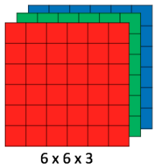
CNN image classifications takes an input image, process it and classify it under certain categories (Eg., Dog, Cat, Tiger, Lion). Computers sees an input image as array of pixels and it depends on the image resolution. Based on the image resolution, it will see h x w x d( h = Height, w = Width, d = Dimension ). Eg., An image of 6 x 6 x 3 array of matrix of RGB (3 refers to RGB values) and an image of 4 x 4 x 1 array of matrix of grayscale image.

Image for post
Figure 1 : Array of RGB Matrix

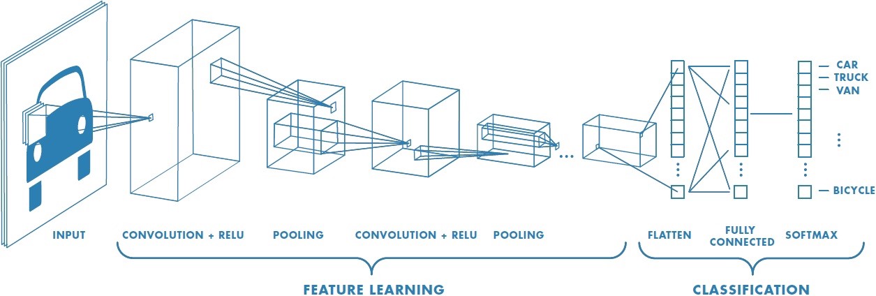
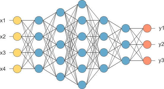
Technically, deep learning CNN models to train and test, each input image will pass it through a series of convolution layers with filters (Kernals), Pooling, fully connected layers (FC) and apply Softmax function to classify an object with probabilistic values between 0 and 1. The below figure is a complete flow of CNN to process an input image and classifies the objects based on values.

Image for post
Figure 2 : Neural network with many convolutional layers

Convolution Layer

Convolution is the first layer to extract features from an input image. Convolution preserves the relationship between pixels by learning image features using small squares of input data. It is a mathematical operation that takes two inputs such as image matrix and a filter or kernel.

Image for post
Figure 3: Image matrix multiplies kernel or filter matrix

Consider a 5 x 5 whose image pixel values are 0, 1 and filter matrix 3 x 3 as shown in below

Image for post
Figure 4: Image matrix multiplies kernel or filter matrix

Then the convolution of 5 x 5 image matrix multiplies with 3 x 3 filter matrix which is called “Feature Map” as output shown in below

Image for post
Figure 5: 3 x 3 Output matrix

Convolution of an image with different filters can perform operations such as edge detection, blur and sharpen by applying filters. The below example shows various convolution image after applying different types of filters (Kernels).

Image for post
Figure 7 : Some common filters

Strides

Stride is the number of pixels shifts over the input matrix. When the stride is 1 then we move the filters to 1 pixel at a time. When the stride is 2 then we move the filters to 2 pixels at a time and so on. The below figure shows convolution would work with a stride of 2.

Image for post
Figure 6 : Stride of 2 pixels

Padding

Sometimes filter does not fit perfectly fit the input image. We have two options:

  • Pad the picture with zeros (zero-padding) so that it fits
  • Drop the part of the image where the filter did not fit. This is called valid padding which keeps only valid part of the image.

Non Linearity (ReLU)

ReLU stands for Rectified Linear Unit for a non-linear operation. The output is ƒ(x) = max(0,x).

Why ReLU is important : ReLU’s purpose is to introduce non-linearity in our ConvNet. Since, the real world data would want our ConvNet to learn would be non-negative linear values.

Image for post
Figure 7 : ReLU operation

There are other non linear functions such as tanh or sigmoid that can also be used instead of ReLU. Most of the data scientists use ReLU since performance wise ReLU is better than the other two.

Pooling Layer

Pooling layers section would reduce the number of parameters when the images are too large. Spatial pooling also called subsampling or downsampling which reduces the dimensionality of each map but retains important information. Spatial pooling can be of different types:

  • Max Pooling
  • Average Pooling
  • Sum Pooling

Max pooling takes the largest element from the rectified feature map. Taking the largest element could also take the average pooling. Sum of all elements in the feature map call as sum pooling.

Image for post
Figure 8 : Max Pooling

Fully Connected Layer

The layer we call as FC layer, we flattened our matrix into vector and feed it into a fully connected layer like a neural network.

Image for post
Figure 9 : After pooling layer, flattened as FC layer

In the above diagram, the feature map matrix will be converted as vector (x1, x2, x3, …). With the fully connected layers, we combined these features together to create a model. Finally, we have an activation function such as softmax or sigmoid to classify the outputs as cat, dog, car, truck etc.,

Image for post
Figure 10 : Complete CNN architecture

Summary

  • Provide input image into convolution layer
  • Choose parameters, apply filters with strides, padding if requires. Perform convolution on the image and apply ReLU activation to the matrix.
  • Perform pooling to reduce dimensionality size
  • Add as many convolutional layers until satisfied
  • Flatten the output and feed into a fully connected layer (FC Layer)
  • Output the class using an activation function (Logistic Regression with cost functions) and classifies images.

In the next post, I would like to talk about some popular CNN architectures such as AlexNet, VGGNet, GoogLeNet, and ResNet.