Camera perception in self-driving cars

Camera perception is one of the most important building blocks in a self-driving car. If radar tells us that something is there and LiDAR helps estimate geometry, the camera gives the system something equally valuable: semantic understanding. A camera can tell us what a traffic light means, what a road sign says, where lane markings curve, whether an object is a pedestrian or a bicycle, and whether a patch of road is drivable or blocked.

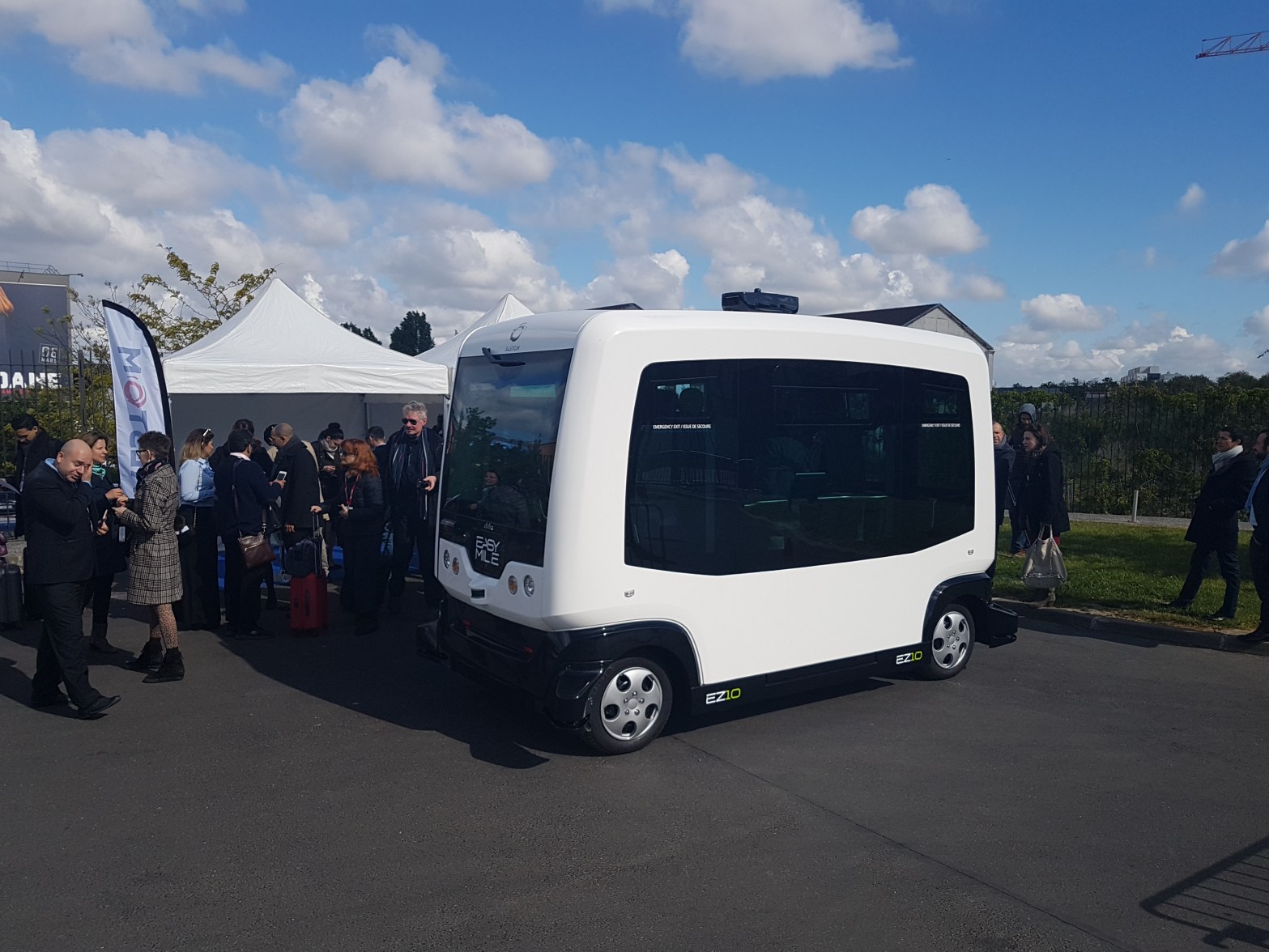
That is why modern autonomous-driving and ADAS systems still rely heavily on cameras, even when they also use radar, LiDAR, ultrasound, and maps. In practice, the camera is often the sensor that gives the richest visual context to the perception stack.

Stereo camera mounted behind a vehicle windshield
Camera modules mounted near the windshield are common in lane keeping, sign recognition, and driver-assistance systems. Source: Wikimedia Commons, Lane assist.jpg.

Why cameras matter so much

A self-driving vehicle does not just need distance. It needs meaning. The system must understand that a small red circle is a stop sign, that a green light means go, that a painted white line marks a lane boundary, and that a person at the curb may step into the road. These are tasks where cameras are especially strong because they capture texture, color, symbols, and shape in dense detail.

In real vehicles, cameras are used for tasks such as:

  • lane detection and lane geometry estimation
  • traffic-light and traffic-sign recognition
  • object detection and classification for cars, trucks, bikes, and pedestrians
  • free-space and drivable-area estimation
  • visual odometry, localization, and mapping
  • parking, surround view, blind-spot coverage, and driver monitoring

The practical advantage is cost and scalability. Cameras are relatively affordable, small, and information-rich, which is why many commercial ADAS platforms are camera-first or at least camera-centric. The limitation is that cameras are sensitive to bad lighting, glare, rain, fog, lens dirt, motion blur, and low texture. So the engineering question is not “camera or other sensors,” but rather “what should the camera do best, and what should be cross-checked by radar, LiDAR, or maps?”

How a camera sees the road

At the mathematical level, most automotive vision pipelines start with the pinhole camera model. A 3D point in the world is projected into a 2D pixel on the image plane. That sounds simple, but in practice you also need to account for lens distortion, focal length, principal point, camera pose, and synchronization with the rest of the vehicle.

Technical figure of the pinhole camera model
The pinhole camera model is the foundation for projection, calibration, and many vision algorithms. Source: Wikimedia Commons, Pinhole camera model technical version.svg.

Three ideas matter here:

  • Intrinsics: focal lengths and principal point that describe how the lens and sensor map light into pixels.
  • Extrinsics: the rotation and translation between the camera and the vehicle frame or world frame.
  • Distortion: radial and tangential effects that bend straight lines unless the image is calibrated and rectified.

If calibration is poor, the whole stack becomes less trustworthy. Lane boundaries drift. Distance estimates become unstable. Multi-camera stitching looks wrong. That is why calibration is not a side issue; it is a core safety and reliability issue.

A small OpenCV-style example for undistortion looks like this:

import cv2 as cv
import numpy as np

image = cv.imread("front_camera.jpg")
camera_matrix = np.array([
    [fx, 0, cx],
    [0, fy, cy],
    [0,  0,  1],
], dtype=np.float32)
dist_coeffs = np.array([k1, k2, p1, p2, k3], dtype=np.float32)

undistorted = cv.undistort(image, camera_matrix, dist_coeffs)

This does not solve perception by itself, but it gives the rest of the pipeline a cleaner and more geometrically meaningful image.

The practical camera pipeline in a self-driving car

Once the image is captured, the perception system usually follows a pipeline similar to this:

  1. Capture and synchronize. Frames must be time-aligned with other cameras, radar, IMU, wheel odometry, and vehicle state.
  2. Calibrate and rectify. Remove distortion and align the image to the vehicle geometry.
  3. Detect and segment. Use classical CV, deep learning, or both to extract lanes, drivable area, traffic lights, signs, and dynamic objects.
  4. Track over time. A single frame is noisy. Multi-frame tracking stabilizes detections and estimates motion.
  5. Estimate geometry. Recover depth from monocular cues, stereo disparity, multi-view triangulation, or fusion with radar/LiDAR.
  6. Fuse and decide. Combine camera output with other sensors and planning logic to support motion decisions.

This is the difference between a demo and a production system. A demo may detect a lane in one image. A production system must maintain stable, low-latency, safety-aware perception under changing weather, different roads, oncoming headlights, and partial occlusion.

What the camera is especially good at

Cameras are the strongest sensor when the system needs semantic detail. Here are the most important examples.

1. Lane understanding

Lane perception is more than finding two white lines. A useful system must estimate lane boundaries, lane center, curvature, merges, splits, missing paint, shadows, and construction zones. In older pipelines, engineers used color thresholding, edge detection, perspective transforms, and Hough lines. In modern systems, deep learning often handles lane segmentation or direct lane representation, but the classical ideas still matter because they explain the geometry and help with debugging.

Example of lane detection with edge and line extraction
A simple lane-detection example showing how edge detection and line fitting can isolate lane candidates. Source: Wikimedia Commons, Lane Detection Example.jpg.

In practice, lane perception supports downstream tasks such as lane keeping, trajectory generation, highway navigation, and safety envelopes around the vehicle.

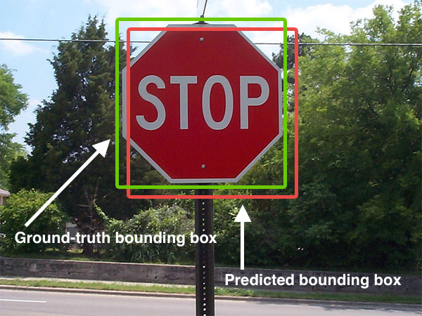
2. Traffic lights and signs

This is where cameras become indispensable. Radar cannot tell whether a light is red or green. LiDAR does not naturally read sign text or arrow direction. Cameras can. That makes them essential for semantic compliance with traffic rules.

A robust traffic-light stack must handle small objects at distance, occlusion, backlighting, LED flicker, and confusing urban scenes. A robust sign-recognition stack must classify signs correctly, but also decide whether a sign applies to the ego lane.

3. Object classification

Knowing that “something exists” is not enough. The planner needs to know whether that object is a pedestrian, cyclist, car, truck, cone, stroller, or road debris. Cameras provide the appearance cues that make this possible.

This is also where temporal reasoning matters. A pedestrian at the sidewalk is not the same as a pedestrian stepping into the crosswalk. The camera gives the appearance; tracking across frames gives intent clues.

4. Visual odometry and localization

Cameras are also useful for localization. By matching features across frames and across maps, the system can estimate motion and refine its position. This becomes even more powerful in stereo or surround-view configurations, or when fused with IMU and map information.

Monocular, stereo, and surround-view setups

Not all camera systems are the same.

  • Monocular camera: cheapest and simplest, strong for classification and lane understanding, weaker for absolute depth unless combined with motion or learned depth cues.
  • Stereo camera: adds geometric depth through disparity, especially useful at short and medium range.
  • Surround-view multi-camera: provides near-360-degree coverage for parking, blind spots, intersections, and urban driving.
Diagram of stereo vision
Stereo vision estimates depth by measuring disparity between left and right images. Source: Wikimedia Commons, Stereovision.gif.

The key stereo idea is simple: a nearby object appears at different horizontal positions in the left and right image. That disparity can be converted to depth. In real systems, however, stereo only works well when calibration and rectification are correct, texture is sufficient, and weather or lighting does not destroy image quality.

Where cameras struggle

It is just as important to understand the limits of cameras.

  • Night and low light: semantic detail drops and noise rises.
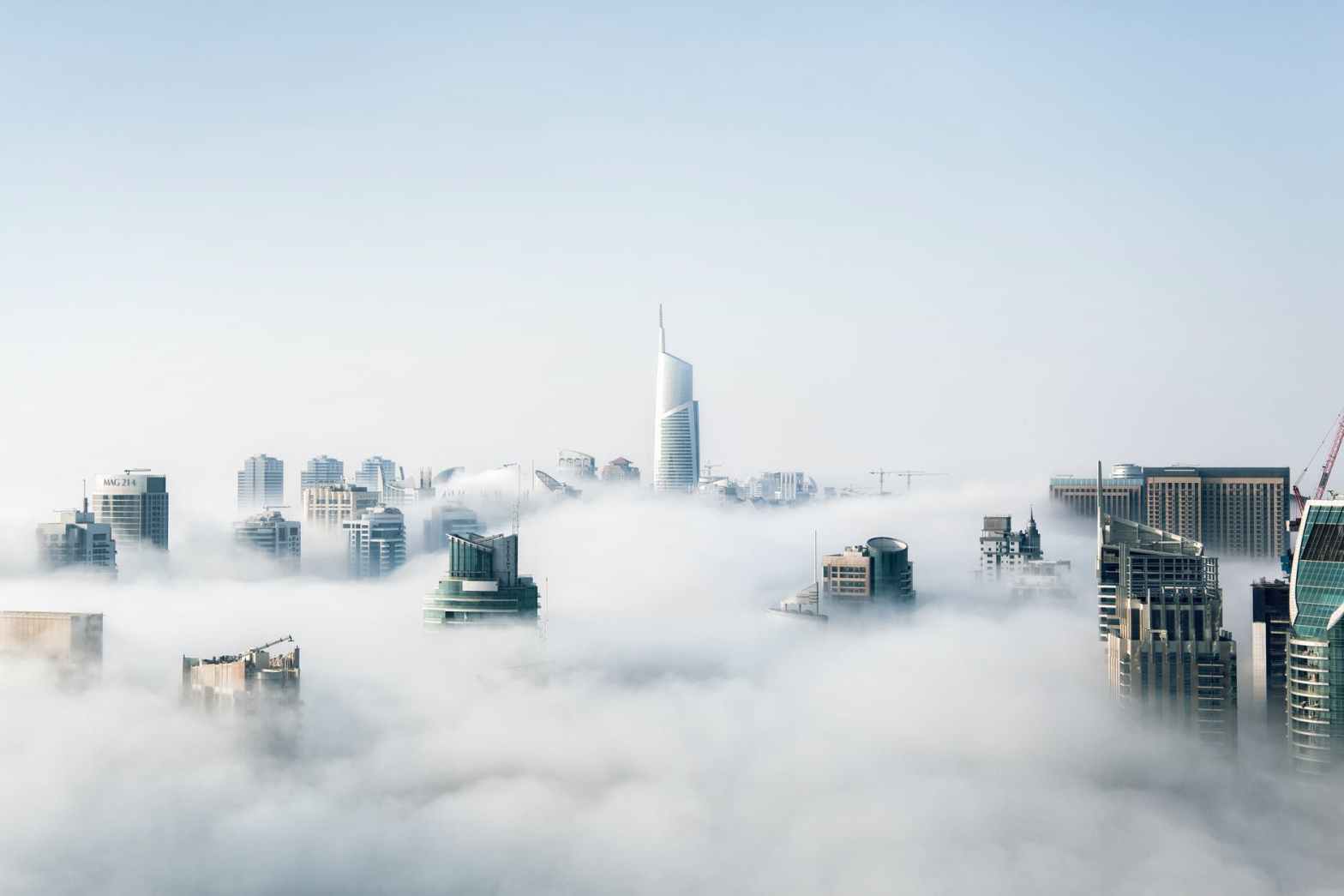
  • Rain, fog, snow, glare: visibility degrades and the model sees less contrast.
  • Dirty or blocked lenses: perception can fail locally even if the rest of the system is healthy.
  • Motion blur and rolling shutter: fast motion distorts geometry.
  • Depth ambiguity: monocular vision is weak at absolute metric depth without additional assumptions or fusion.

That is why production systems rarely trust a camera alone for all situations. Camera-first makes sense for semantics and scale, but sensor fusion still matters for robustness.

Why camera-first still makes sense

Even with those weaknesses, cameras remain central because they match several practical engineering goals at once:

  • they capture dense visual information
  • they are cheaper and easier to scale than high-end active sensors
  • they support the semantic tasks that every road-legal system must solve
  • they fit both ADAS and higher-autonomy stacks

That is why many commercial systems use a camera-first or camera-centric architecture, then add radar, LiDAR, maps, and driver monitoring where the safety case demands it.

A practical engineering checklist

If you are building or evaluating a camera-based perception stack, these are the questions that matter most:

  • How stable is calibration over time, temperature, vibration, and mounting changes?
  • What happens under glare, nighttime, rain, and lens contamination?
  • How much latency exists from image capture to decision output?
  • Which tasks are vision-only, and which require fusion?
  • How is uncertainty represented and passed to planning?
  • Does the system fail gracefully when the image quality drops?

Those questions usually separate a classroom demo from an automotive-grade perception module.

Conclusion

The camera is not just a passive eye on a self-driving car. It is the main source of semantic road understanding. It tells the system what the world means, not just where something is. That makes cameras essential for lane understanding, traffic-light recognition, sign reading, object classification, localization, and many driver-assistance functions.

At the same time, good camera perception depends on careful calibration, stable geometry, robust learning models, temporal tracking, and realistic handling of bad-weather and low-light failures. In other words, the power of cameras in autonomous driving is real, but it only becomes useful when the full engineering pipeline around the camera is strong.

References

System integration for self-driving cars

Self-driving systems are often explained as separate modules: localization, perception, prediction, planning, and control. That modular view is useful, but it can also be misleading. A real autonomous-driving stack does not succeed because one block is excellent in isolation. It succeeds because the blocks exchange the right information, at the right time, with the right assumptions.

That is what system integration really means. It is the engineering discipline of connecting sensing, localization, maps, planning, control, and vehicle interfaces into one coherent pipeline that can operate safely under real-world timing and uncertainty constraints.

Why integration matters more than slideware

A strong perception model is not enough if localization drifts. A good planner is not enough if control cannot follow the trajectory. A precise controller is not enough if the vehicle interface delays commands or clips them unexpectedly. In practice, many failures appear at the boundaries between modules rather than inside a single algorithm.

That is why mature autonomous-driving projects place so much emphasis on interfaces, diagnostics, synchronization, fallback behavior, and system architecture.

The major building blocks

A practical self-driving stack usually contains these major layers:

  1. Sensing: cameras, LiDAR, radar, IMU, GNSS, wheel odometry, and vehicle-state signals.
  2. Localization: estimate current pose, velocity, and acceleration.
  3. Perception: detect lanes, objects, traffic lights, free space, and obstacles.
  4. Prediction: estimate how other agents may move next.
  5. Planning: choose a safe route, path, and trajectory.
  6. Control: convert the planned trajectory into steering, acceleration, and braking commands.
  7. Vehicle interface: deliver those commands safely to the actual platform.

These blocks are familiar, but the real work is in their coordination.

How information flows through the system

A useful integrated stack behaves like a pipeline with feedback, not like a row of isolated boxes.

sensors
    -> localization
    -> perception
    -> prediction
    -> planning
    -> control
    -> vehicle interface

diagnostics and state feedback
    -> monitor health, uncertainty, delays, and fallback modes

Autoware’s architecture documents make this dependency clear. Planning depends on information from localization, perception, and maps. Control depends on the reference trajectory from planning. Localization itself may depend on LiDAR maps, IMU data, and vehicle velocity. If any upstream information is stale or unstable, the downstream behavior degrades.

Localization is not just a coordinate estimate

In an integrated system, localization must provide more than a rough pose. It must provide:

  • pose in the map frame
  • velocity and acceleration estimates
  • covariance or confidence information
  • timestamps that align with the rest of the pipeline

That information is consumed directly by planning and control. If localization lags behind reality or reports unstable motion, planning may generate a trajectory that is already outdated.

Perception must produce planning-ready outputs

Perception often gets too much attention as a standalone benchmark problem. But in a vehicle stack, the most important question is not whether perception is impressive in a paper. It is whether it produces the exact outputs planning needs.

For example, planning may need:

  • detected objects with stable tracks
  • obstacle information for emergency stopping
  • occupancy information for occluded regions
  • traffic-light recognition tied to the relevant route

This is one reason Autoware’s documentation describes planning inputs very carefully: the planner relies on structured, timely, route-relevant environment information, not on generic detections alone.

Planning and control are tightly linked

Planning produces a trajectory, but that trajectory is only useful if control can execute it. Control modules need trajectories that are smooth, physically feasible, and consistent with the actual vehicle model. If the planner outputs unrealistic curvature or aggressive accelerations, the controller either fails or compensates in ways that create instability.

Autoware’s control design documents highlight exactly this relationship: control follows the reference trajectory from planning and converts it into target steering, speed, and acceleration commands. That is a clean architectural separation, but it still requires the planner and controller to agree on timing, kinematics, and limits.

What system integration usually includes

In practice, system integration is not only about software wiring. It includes:

  • message contracts and interface definitions
  • coordinate frames and transforms
  • sensor synchronization
  • health monitoring and diagnostics
  • latency budgeting
  • fallback and degradation strategies
  • vehicle-specific adaptation layers

That last point matters. A generic autonomy stack often outputs abstract commands such as target speed, acceleration, and steering angle. A vehicle-specific adapter then maps those commands to the actual hardware interface. This is another place where integration quality matters enormously.

Common integration failures

Some of the most important failures in autonomous systems are integration failures, not algorithmic failures:

  • timestamps from different sensors do not align
  • map and vehicle frames are inconsistent
  • perception outputs are too noisy for planning
  • control receives trajectories it cannot track smoothly
  • diagnostics do not catch degraded modules quickly enough
  • vehicle adapters change behavior relative to what higher layers expect

These problems can make a technically strong stack behave unpredictably in the field.

What a good integrated stack looks like

A well-integrated self-driving stack tends to have these qualities:

  • clear interfaces between modules
  • consistent coordinate frames and timing
  • explicit uncertainty and diagnostics
  • modular components that can still be validated end-to-end
  • graceful degradation when one sensor or module weakens

In other words, good system integration does not remove modularity. It makes modularity usable in a real vehicle.

A practical checklist

If I were reviewing a self-driving integration effort, I would ask:

  • Which modules define the system time base and synchronization policy?
  • How are localization confidence and perception uncertainty passed downstream?
  • What happens when planning receives stale or inconsistent inputs?
  • Can control reject trajectories it cannot safely follow?
  • How is the vehicle interface validated against actual hardware response?
  • What diagnostics trigger fallback or minimal risk behavior?

Those questions often reveal the real maturity of the stack faster than demo footage does.

Conclusion

System integration is what turns separate autonomy modules into an actual self-driving system. Localization, perception, planning, control, and the vehicle interface must agree not only on data format, but also on timing, confidence, physical limits, and safety behavior. That is why system integration is not a final polish step. It is one of the core engineering problems in autonomous driving.

References

Computer vision and sensors

Autonomous systems do not rely on a single technology. They work because several layers of perception support each other. Computer vision extracts visual structure, deep learning helps recognize patterns and objects, and sensors provide the raw measurements needed to understand the environment.

Computer Vision vs Deep Learning

These two ideas are related, but not identical. Traditional computer vision focuses on geometry, edges, features, transformations, calibration, and image processing. Deep learning focuses on learning complex patterns from data, often through neural networks.

In practice, modern systems use both. Geometry still matters, and learned perception has become essential.

Why Sensors Matter

A camera gives rich visual data, but no single sensor is enough in all conditions. Real autonomous systems often combine:

  • cameras for semantics and rich scene information,
  • LiDAR for geometry and depth structure,
  • radar for robustness in difficult weather,
  • IMU and odometry for short-term motion tracking.

A Practical Pipeline

A perception stack in an autonomous vehicle may look like this:

  1. Cameras capture road scenes.
  2. Deep models detect lanes, vehicles, pedestrians, and signs.
  3. LiDAR or radar improves distance estimation and object consistency.
  4. Sensor fusion tracks objects over time.
  5. The planning stack uses this interpreted scene to make decisions.

Where Traditional Vision Still Helps

  • camera calibration,
  • stereo depth estimation,
  • visual odometry,
  • image rectification,
  • pose estimation and geometry-based reasoning.

Where Deep Learning Adds Value

  • object detection,
  • semantic segmentation,
  • lane understanding,
  • driver or pedestrian behavior cues,
  • end-to-end learned scene interpretation.

Final Thoughts

The strongest autonomous systems are not built by choosing between classical computer vision and deep learning. They are built by using the right combination of sensing, geometry, learning, and engineering discipline for the task at hand.

Yolo for real-time detection

YOLO, short for You Only Look Once, changed how many engineers think about object detection. Earlier detection systems often used multi-stage pipelines that proposed regions first and classified them later. YOLO reframed detection as a direct prediction problem: take an image, run one forward pass, and predict bounding boxes plus class scores quickly enough for real-time use.

That design choice made YOLO especially attractive in robotics, video analytics, and autonomous systems, where latency matters as much as raw accuracy.

Bounding boxes for object detection example
Object detection is not just classification. The model must also localize the object with a useful bounding box. Source: Wikimedia Commons, Intersection over Union – object detection bounding boxes.jpg.

What problem YOLO solves

Image classification answers a simple question: what is in this image? Detection answers a harder one: what objects are present, where are they, and which class belongs to each box?

That difference matters in real systems. A vehicle or robot does not only need to know that a scene contains a pedestrian. It needs to know where the pedestrian is, how that person moves across frames, and whether the detection is stable enough to influence planning.

YOLO became popular because it made this detection step fast and practical at scale.

Why YOLO became influential

There are three main reasons YOLO spread so widely:

  • Speed: real-time inference made it attractive for video and edge deployment.
  • Simplicity: a single unified detector was easier to explain and deploy than older multi-stage systems.
  • Strong engineering ecosystem: later implementations and tooling made training, exporting, and deployment more accessible.

Over time, the YOLO family evolved a lot. Anchor strategies changed, backbones improved, post-processing changed, and modern variants added tasks such as segmentation, pose, tracking, and oriented boxes. But the core identity remained: detection should be fast enough to use in real systems.

How YOLO works at a practical level

Conceptually, YOLO takes an image and predicts object locations and categories in one inference path. A modern pipeline usually includes:

  1. image resize and normalization
  2. feature extraction with a backbone network
  3. multi-scale detection heads
  4. confidence scoring and class prediction
  5. post-processing to remove duplicate boxes

The exact architecture depends on the version you use, but the operational idea is stable: produce detections quickly enough for downstream systems to react.

from ultralytics import YOLO

model = YOLO("yolo11n.pt")
results = model("street_scene.jpg")

for result in results:
    for box in result.boxes:
        print(box.cls, box.conf, box.xyxy)

The code above looks simple, but the real engineering work is often around dataset quality, deployment constraints, label consistency, camera setup, and tracking across frames.

Where YOLO fits in a larger system

YOLO is rarely the whole perception stack. In a deployed system it usually feeds into something larger:

  • multi-object tracking
  • sensor fusion
  • risk estimation
  • behavior planning
  • alerting or actuation logic

For example, in an autonomous-driving context, YOLO-style detection may identify vehicles, pedestrians, bikes, and traffic cones. But planning still needs temporal tracking, motion prediction, and safety rules before it can turn those detections into driving decisions.

What YOLO is especially good at

YOLO tends to work well when you need:

  • fast detection on live video
  • compact deployment on edge hardware
  • simple integration into monitoring or robotics pipelines
  • good tradeoffs between speed and accuracy

This is why it appears so often in drones, traffic monitoring, warehouse robots, industrial safety, and smart-camera systems.

Where YOLO is not enough by itself

Even a strong detector has limits. YOLO alone does not solve:

  • precise depth estimation
  • fine-grained pixel segmentation
  • long-term tracking identity under heavy occlusion
  • full scene understanding for planning
  • robust performance under severe domain shift without retraining

That is why practical systems usually pair detection with tracking, segmentation, map context, or other sensors.

Real engineering concerns

If you plan to deploy YOLO in a real product, the hard questions are usually not about the marketing benchmark. They are about:

  • label quality and class definitions
  • how often false positives appear in safety-critical scenes
  • how small distant objects can be while still being detected
  • latency on the exact target hardware
  • nighttime, rain, motion blur, or camera vibration
  • monitoring drift after deployment

In many teams, the biggest performance gains come from better data and better deployment choices, not from chasing a new model name every week.

Conclusion

YOLO became influential because it made object detection fast, practical, and easy to integrate into real systems. It remains a strong choice when engineers need real-time perception on images or video. But the best way to use YOLO is to treat it as one reliable module inside a broader perception stack, not as the full system by itself.

References

How self-driving cars work

A self-driving car is not one algorithm and not one sensor. It is a layered system that combines perception, localization, prediction, planning, and control so the vehicle can understand traffic scenes and act safely in real time.

1. Perception

Perception is responsible for answering the question: What is around the car? A self-driving stack may use cameras, LiDAR, radar, ultrasonic sensors, and GPS/IMU inputs. Perception algorithms detect lanes, vehicles, pedestrians, cyclists, traffic signs, and traffic lights.

Modern systems often combine deep learning with geometric tracking. For example, a camera may detect a pedestrian while LiDAR refines shape and distance. Sensor fusion improves reliability because no single sensor is perfect in all conditions.

2. Localization

Localization answers: Where is the car? GPS alone is usually not accurate enough for lane-level autonomy, so self-driving cars often combine GNSS, IMU, wheel odometry, HD maps, and LiDAR or camera-based matching. The goal is to maintain a precise estimate of position and orientation.

3. Prediction

Other road users move unpredictably. Prediction estimates what they may do next. A vehicle ahead may brake. A pedestrian may step onto the road. A cyclist may merge into the lane. The system therefore predicts future trajectories and uncertainties, not only current positions.

4. Behavior Planning

Behavior planning decides the high-level action: keep lane, stop, yield, overtake, or change lanes. It converts traffic understanding into a driving decision that respects safety and road rules.

5. Motion Planning

Once the system knows what behavior it wants, it needs a feasible trajectory. Motion planning generates a path that is safe, smooth, and physically possible for the vehicle. It considers curvature, speed, nearby obstacles, and passenger comfort.

6. Control

The control layer converts the planned trajectory into steering, throttle, and brake commands. Controllers such as PID, MPC, or LQR help the car track the planned path while remaining stable and responsive.

A Driving Example

Imagine the car approaches a slower vehicle in the same lane:

  1. Perception detects the vehicle ahead and estimates distance.
  2. Localization places the ego car accurately on the map.
  3. Prediction estimates whether the other vehicle will continue straight or slow further.
  4. Behavior planning decides whether to follow or change lane.
  5. Motion planning creates a smooth and safe trajectory.
  6. Control executes the maneuver.

Why Building a Self-Driving Car Is Difficult

  • Real traffic is uncertain and full of corner cases.
  • Sensors are noisy and can fail.
  • Decisions must be made in real time.
  • Safety validation is extremely demanding.

Final Thoughts

The best way to understand self-driving technology is to see it as a systems engineering problem. Each module matters, but what matters most is how well the modules work together under real-world conditions.

Vision-based navigation in practice

Vision-based navigation uses cameras to estimate motion, understand the environment, and help a robot or vehicle move safely through space. It is attractive because cameras are relatively cheap, lightweight, and rich in detail. A single frame can contain landmarks, lane markings, free space, signs, texture, and semantic cues that other sensors may not capture as naturally.

But camera-based navigation is not simply “look at an image and drive.” A practical navigation stack needs stable calibration, time synchronization, robust pose estimation, and a way to recover when the scene becomes ambiguous.

Camera module near windshield for assisted driving
Cameras mounted near the windshield often support lane keeping, road understanding, and navigation cues. Source: Wikimedia Commons, Lane assist.jpg.

What vision-based navigation really does

At a practical level, vision-based navigation answers three questions:

  • Where am I?
  • How am I moving?
  • What is around me, and where can I go next?

Depending on the platform, the answer may rely on visual odometry, landmark tracking, semantic road understanding, stereo depth, or full SLAM. In an indoor robot, the system may rely on features and loop closure. In a road vehicle, it may use cameras for lane geometry, localization cues, and scene semantics while radar, GNSS, IMU, and maps handle complementary tasks.

The core pipeline

A practical camera-navigation pipeline often looks like this:

  1. Capture synchronized images from one or more calibrated cameras.
  2. Extract visual information such as features, edges, segments, landmarks, or semantic masks.
  3. Estimate motion using frame-to-frame correspondences, optical flow, stereo disparity, or learned motion models.
  4. Build or update a map of landmarks, occupancy, or semantic structure.
  5. Fuse with other sensors such as IMU, wheel odometry, GNSS, LiDAR, or radar.
  6. Provide pose and environment estimates to planning and control.

That pipeline may sound straightforward, but every stage can fail if the image stream is noisy, blurred, poorly synchronized, or visually repetitive.

Visual odometry and SLAM

Two ideas appear in almost every camera-navigation system: visual odometry and SLAM.

Visual odometry estimates the motion of the camera by tracking how the scene changes across frames. It is local and continuous. It tells the system how it moved over the last short period of time.

SLAM, or simultaneous localization and mapping, goes further. It tries to build a consistent map while also using that map to improve localization. Loop closure is especially important here. If the robot revisits a known place, the system can reduce drift and relocalize more accurately.

Systems such as ORB-SLAM became influential because they showed that a camera-only pipeline could estimate trajectory in real time across a wide range of environments. Newer systems expanded this idea to stereo, RGB-D, and visual-inertial settings.

navigation stack
    -> synchronized camera frames
    -> feature tracking or semantic perception
    -> relative pose estimate
    -> map update / loop closure
    -> fused state estimate
    -> planner and controller

What cameras are good at in navigation

Cameras are especially useful when the platform needs semantic context in addition to geometry.

  • Road structure: lanes, curbs, drivable area, intersections, merges, and signs.
  • Landmarks: textured features, repeated landmarks, or learned place descriptors.
  • Obstacle understanding: identifying whether something is a car, pedestrian, bike, or static structure.
  • Localization support: map matching and relocalization from known visual features.

This semantic richness is why cameras remain central in ADAS, delivery robots, warehouse systems, and many research platforms.

Monocular, stereo, and multi-camera navigation

Not all vision-based navigation systems see the world the same way.

  • Monocular: lowest cost and simplest hardware, but scale is ambiguous without motion priors or fusion.
  • Stereo: adds depth through disparity, making pose and obstacle reasoning more stable.
  • Multi-camera surround view: improves coverage at intersections, blind spots, and tight maneuvers.
Stereo vision depth concept
Stereo vision converts left-right image disparity into depth cues that improve navigation and obstacle reasoning. Source: Wikimedia Commons, Stereovision.gif.

Monocular systems can still work very well, especially with IMU fusion, but stereo or multi-camera setups reduce ambiguity when metric depth matters.

Why fusion matters

Camera navigation alone can be impressive, but robust deployed systems almost always fuse vision with other sources of information. An IMU helps stabilize short-term motion estimation. Wheel odometry provides a useful prior for ground robots. GNSS helps with large-scale outdoor localization. LiDAR or radar can add stronger geometric constraints under difficult lighting conditions.

The engineering goal is not to replace every other sensor with cameras. The goal is to let cameras contribute what they do best and rely on fusion when ambiguity grows.

Common failure modes

Vision-based navigation fails for understandable reasons, and those failure modes should shape the system design:

  • low light or night scenes reduce usable detail
  • glare, rain, fog, and dirty lenses degrade image quality
  • textureless walls or roads reduce feature quality
  • dynamic crowds or heavy traffic can confuse motion estimation
  • repetitive patterns create false matches
  • timing and calibration errors break the geometry

If a system does not monitor these conditions, it may produce confident but wrong poses. That is one of the main reasons why state estimation and uncertainty reporting matter so much.

A practical engineering checklist

When evaluating a vision-navigation stack, I would check these points first:

  • How well is camera calibration maintained over time?
  • What is the end-to-end latency from sensor capture to pose output?
  • How much drift appears before loop closure or relocalization?
  • How does the system behave in low-texture or high-dynamic scenes?
  • Which modules depend on pure vision and which depend on fusion?
  • Can the planner detect when localization confidence drops?

Those questions reveal much more than a single demo video.

Conclusion

Vision-based navigation is powerful because cameras provide both geometry and semantics. They help a system estimate motion, understand roads or indoor structure, recognize landmarks, and support localization over time. But reliable navigation requires more than a neural network. It requires calibration discipline, temporal reasoning, mapping, and sensible fusion with other sensors. That is what turns camera-based navigation from a nice demo into a dependable part of a robotics or autonomous-driving stack.

References

Ibm doors for requirements engineers

IBM DOORS is a requirements management tool widely used in industries where traceability, documentation, and process discipline matter, such as automotive, aerospace, rail, and safety-critical systems. For many software engineers, it feels very different from the more informal workflow of modern application development, but it exists for an important reason.

Why Requirements Tools Matter

In large engineering projects, requirements are not just notes. They must be reviewed, versioned, linked, and verified. A change in one requirement can affect architecture, testing, compliance, and delivery plans. Tools like DOORS help teams manage that complexity more systematically.

What DOORS Is Used For

  • capturing system and software requirements,
  • organizing requirements into modules,
  • creating links between parent and child requirements,
  • supporting traceability from requirement to test case,
  • tracking reviews and controlled changes.

A Practical Example

Imagine an automotive braking subsystem. A system-level requirement may define a safety response time. That requirement can be linked to lower-level software requirements, design documents, test cases, and validation evidence. If the parent requirement changes, teams can quickly identify what downstream artifacts are affected.

Why Engineers Often Struggle with It

DOORS is powerful, but it can feel heavy if a team is used to moving fast without strong documentation rules. The tool works best when the project genuinely needs structure, auditability, and long-lived engineering records.

Good Practices

  • Write requirements that are specific and testable.
  • Avoid combining several ideas in one requirement.
  • Keep traceability meaningful rather than creating links only for process optics.
  • Review change impact carefully before updating baselines.

Final Thoughts

IBM DOORS is not exciting in the same way as AI or cloud platforms, but it is important in serious engineering environments. If you understand why traceability matters, you understand why tools like DOORS continue to play a major role in large technical programs.

Occupancy grid maps in practice

Occupancy grid maps are one of the most practical map representations in robotics. They divide space into cells and estimate whether each cell is free, occupied, or still unknown. That sounds simple, but the representation is powerful because it turns noisy sensor measurements into a structure that planning, localization, and obstacle reasoning can use directly.

Occupancy grids remain popular because they are conceptually clear, easy to update incrementally, and compatible with a wide range of sensors and algorithms.

The basic idea

Imagine covering the world with a 2D chessboard. Every square stores the current belief about whether that patch of space contains an obstacle. If the robot sees repeated evidence that a cell is blocked, the occupancy probability rises. If the robot repeatedly observes that a cell is clear, the probability falls. Cells that have not been observed remain unknown.

This representation is attractive because it makes uncertainty explicit. The map does not pretend to know the world perfectly. It stores a belief that can change as new measurements arrive.

Why occupancy grids matter

Occupancy grids are useful because they bridge sensing and action. Raw LiDAR or sonar readings are hard for a planner to use directly. A grid map converts those measurements into a spatial memory that answers practical questions such as:

  • Which nearby cells are clearly free?
  • Where are likely obstacles?
  • Which regions remain unknown or poorly observed?
  • Is there a safe corridor from the current pose to the goal?

That makes occupancy grids especially valuable in mobile robotics, autonomous navigation, and obstacle avoidance.

How sensor updates work

The most common formulation updates each cell probabilistically from incoming sensor data. Laser scans, depth sensors, or range observations are traced into the map:

  • cells along the beam are often reinforced as free
  • the end point is reinforced as occupied if an obstacle was detected
  • cells beyond the obstacle remain unknown because the sensor did not see through it

Many systems use a log-odds update because it makes repeated Bayesian updates efficient. Instead of storing raw probabilities directly, the map stores a transformed value that can be incremented or decremented more easily as evidence accumulates.

for each laser beam:
    mark traversed cells as more likely free
    mark impact cell as more likely occupied
    keep unobserved cells unknown

That small pattern is the heart of many practical grid-mapping systems.

Resolution is a real engineering tradeoff

Occupancy grids look straightforward until you choose the cell size. Resolution affects almost everything:

  • finer cells capture more detail
  • coarser cells reduce memory and compute load
  • planning cost often scales badly as resolution becomes too fine
  • small errors and sensor noise can become exaggerated at very high resolution

MRPT’s occupancy-grid notes highlight this tradeoff clearly: many operations scale with the square of the inverse resolution. That means halving the cell size can increase computational cost dramatically.

So the “best” resolution is not the finest possible one. It is the one that matches the robot size, sensor noise, and planning needs.

How grids support planning

Once the map stores free and occupied cells, a planner can search for safe paths. The simplest approach is to inflate obstacles by the robot radius, then run a path-planning algorithm over the remaining free cells. This is why occupancy grids are so practical: they convert navigation into a structured search problem.

MRPT’s planning examples show this nicely. A circular robot can plan over a 2D occupancy grid after obstacle growth, using value iteration or similar methods to find a path toward the goal.

This works well for many indoor or moderately structured environments, even if the final motion planner later refines the path more smoothly.

Where occupancy grids are strong

  • simple and intuitive representation
  • works naturally with range sensors
  • supports incremental updates over time
  • easy to use for planning and collision checking
  • keeps uncertainty visible through free, occupied, and unknown space

Where occupancy grids become limited

Despite their usefulness, occupancy grids also have limitations:

  • large maps consume significant memory
  • fixed resolution may waste detail in some areas and lose detail in others
  • 2D grids do not represent height or overhangs well
  • dynamic environments require frequent updates and clearing
  • the map alone does not explain object identity or semantics

These limitations are why teams sometimes move to hierarchical structures such as octomaps for 3D, or add semantic layers on top of the occupancy representation.

Occupancy grids in modern autonomous systems

Occupancy grids are still relevant in modern autonomy stacks. Autoware’s perception and planning documentation explicitly includes occupancy-map information as an input for planning. That makes sense: even if object detectors and lane models are available, a planner still benefits from a spatial representation of drivable, blocked, and occluded areas.

In other words, occupancy grids are not outdated. They remain one of the cleanest ways to represent navigable space under uncertainty.

A practical checklist

If I were reviewing a grid-mapping system, I would look at:

  • cell resolution and its effect on runtime
  • sensor model assumptions used for free and occupied updates
  • how unknown space is handled by planning
  • whether dynamic obstacles are cleared correctly
  • how obstacle inflation matches robot geometry
  • whether 2D is sufficient or a 3D map is required

These questions usually matter more than the visualization itself.

Conclusion

Occupancy grid maps remain a foundational tool in robotics because they turn uncertain sensor data into a representation that planners and navigation systems can actually use. Their strength lies in simplicity, probabilistic updates, and close compatibility with path planning. Their weaknesses appear when environments become very large, highly dynamic, or deeply three-dimensional. But as a practical engineering tool, occupancy grids still matter a great deal.

References

Autonomous navigation basics

Autonomous navigation is the ability of a robot or vehicle to move through an environment safely and purposefully without continuous human control. In practice, that means much more than following a path. A useful autonomous system has to understand where it is, what surrounds it, where it should go, and how to move there safely.

The Core Pipeline

Although implementations differ, most navigation systems can be understood through a few major blocks:

  • Perception: sensing the environment using cameras, LiDAR, radar, ultrasound, GPS, IMU, or wheel encoders.
  • Localization: estimating the current position and orientation of the robot.
  • Mapping: building or using a representation of the world.
  • Planning: deciding where to go and how to get there.
  • Control: generating steering, throttle, brake, or wheel commands to follow a trajectory.

Perception

No navigation system can work well without useful sensor input. Cameras provide rich visual information, LiDAR provides accurate geometric structure, radar performs well in difficult weather, and IMU sensors help with short-term motion tracking. In many real systems, sensor fusion is essential because each sensor has strengths and weaknesses.

Localization

A robot must know where it is before it can move intelligently. Localization may rely on GPS outdoors, but in indoor or high-precision environments it often depends on SLAM, particle filters, Kalman filters, or map-based matching. Even a strong planner becomes useless if the position estimate drifts too far from reality.

Mapping

Some robots navigate in a prebuilt map, while others build a map online. Common map types include occupancy grids, feature maps, lane maps, topological graphs, and semantic maps. The right representation depends on the environment and task. A warehouse robot does not need the same map structure as a self-driving car in urban traffic.

Planning

Planning can be divided into layers:

  • Global planning: choose a route from start to destination.
  • Behavior planning: decide actions such as stopping, yielding, or changing lanes.
  • Local planning: generate a feasible short-horizon trajectory around obstacles.

Algorithms may include A*, Dijkstra, RRT, lattice planners, optimization-based methods, or behavior rules depending on the system.

Control

Once a trajectory exists, the controller turns it into actual motion. Common controllers include PID, pure pursuit, Stanley, LQR, and MPC. The choice depends on dynamics, accuracy requirements, and computational constraints.

A Real Example

Consider an autonomous delivery robot in a campus environment:

  1. It uses GNSS and IMU outdoors, plus LiDAR for obstacle detection.
  2. It localizes against a map of pathways and building entrances.
  3. It plans a global route to the target building.
  4. It adjusts locally to avoid pedestrians and parked bicycles.
  5. Its controller tracks the resulting path while keeping speed smooth and safe.

Why Autonomous Navigation Is Hard

  • Sensor noise and drift are unavoidable.
  • The world changes: people move, objects appear, weather varies.
  • Planning must balance safety, comfort, efficiency, and real-time constraints.
  • The full system only works if the modules interact reliably.

Final Thoughts

Autonomous navigation is not a single algorithm. It is a system problem that combines sensing, estimation, decision-making, and control. Understanding the interfaces between those layers is what turns theory into a working robot or vehicle.