Canny edge detection is one of those classic computer vision tools that still deserves attention. Even in an era dominated by deep learning, engineers keep returning to Canny because it is fast, interpretable, and useful for building baselines, debugging camera pipelines, and extracting geometric structure from images.
It is especially valuable when you want to highlight boundaries such as lane markings, road edges, object contours, or structural lines before running later stages of a pipeline.
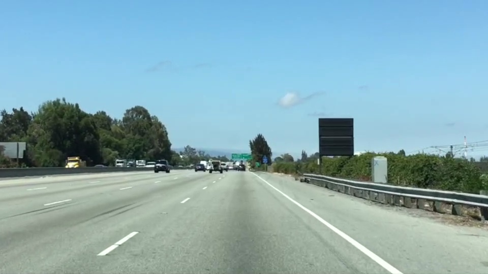
A simple lane pipeline often starts with edge extraction before fitting lines or estimating road structure. Source: Wikimedia Commons, Lane Detection Example.jpg.
Why Canny still matters
Most raw images contain far more information than a geometric pipeline needs. Canny helps reduce that image to a sparse set of likely boundaries. That makes it useful in applications such as:
lane detection prototypes
document and industrial inspection
line or contour extraction
preprocessing for feature-based pipelines
debugging lighting and contrast issues in camera systems
It is not a full perception system, but it is often a strong first step when the engineer wants structure rather than semantics.
How the algorithm works
Canny is a multi-stage edge detector. Its power comes from the fact that it does not simply compute gradients and stop there. It also tries to suppress noise and keep only meaningful, thin edges.
Noise reduction: smooth the image, usually with a Gaussian filter.
Gradient computation: estimate intensity changes, often with Sobel operators.
Non-maximum suppression: keep only local maxima so the edge stays thin.
Hysteresis thresholding: use lower and upper thresholds to decide which edges survive.
This last step is one reason Canny stays practical. Weak responses can still survive if they connect to strong edges, which often preserves useful line structure while discarding isolated noise.
What the thresholds really do
Most failures with Canny are not about the algorithm itself. They are about poor threshold choices.
If the thresholds are too low, noise floods the result.
If the thresholds are too high, meaningful boundaries disappear.
If the image is not smoothed well, texture and noise create unstable edges.
That is why Canny tuning is often scene-dependent. A bright daytime road scene may support different thresholds than a nighttime wet road.
That simple code hides an important practical truth: preprocessing usually matters as much as the call to cv.Canny() itself.
How engineers use Canny in lane detection
Canny became a familiar tool in beginner autonomous-driving projects because it works well as part of a classical lane-detection pipeline. A common sequence is:
convert the image to grayscale
blur to reduce noise
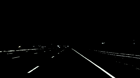
run Canny to extract edges
apply a region of interest mask
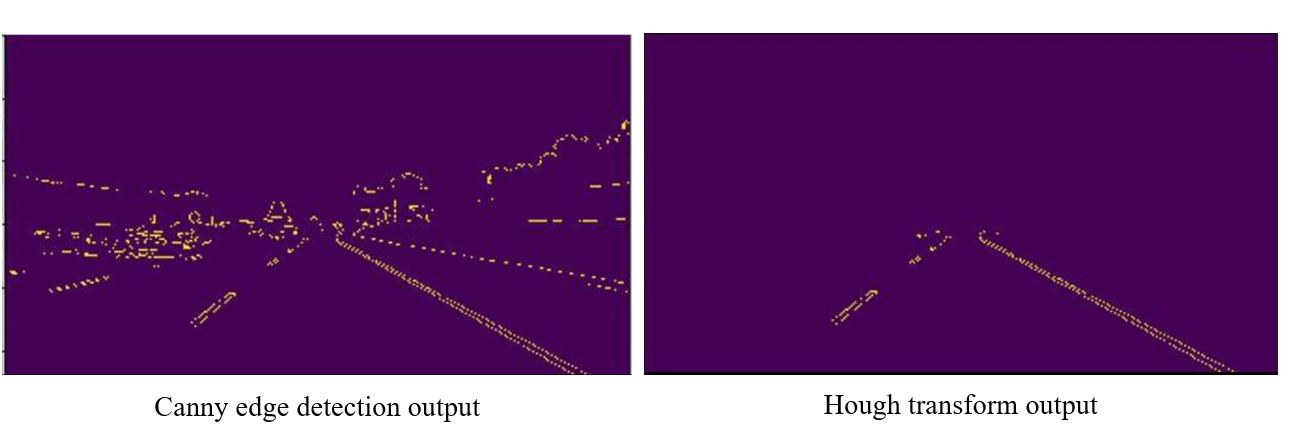
fit candidate lane lines with a Hough transform
Canny often plays the role of edge extractor inside a broader lane-detection pipeline. Source: Wikimedia Commons, Lane Detection Algorithm.svg.
This does not solve all real road cases, but it teaches the underlying geometry clearly and remains useful for debugging modern lane systems.
Where Canny is strong
fast and cheap to run
easy to interpret visually
good for highlighting sharp structure
useful in classical pipelines and for debugging learned models
Where Canny is weak
it does not understand semantics
it is sensitive to threshold selection
it struggles with shadows, glare, and heavy texture
it cannot decide whether an edge belongs to a lane, a crack, or a shadow by itself
That is why modern systems usually combine Canny-like geometric ideas with learning-based perception when the scene is complex.
A practical way to use it today
Even if your final product relies on neural networks, Canny still has value. I would use it for:
building a classical baseline quickly
validating whether the camera image quality is good enough for geometry
checking if calibration or blur is destroying useful structure
explaining perception stages to new engineers on the team
It is one of those rare classical methods that remains useful both educationally and operationally.
Conclusion
Canny edge detection still matters because it turns a noisy image into a much clearer geometric signal. It is not a semantic perception tool, but it remains valuable for lane-finding pipelines, contour extraction, debugging, and building intuition about how vision systems interpret structure. For many engineering teams, Canny is still one of the quickest ways to understand what the camera can and cannot see.
Region masking is one of the simplest ideas in computer vision, yet it solves a very practical problem: most of the pixels in an image are irrelevant to the task you care about. If you are trying to detect lane lines from a front-facing road camera, the sky, nearby buildings, dashboard reflections, and other distant objects often add noise instead of useful signal.
Region masking fixes that by keeping only the part of the image where lane structure is likely to appear. In other words, it tells the pipeline: “Look here first, and ignore the rest.”
Lane-detection pipelines often restrict processing to a selected road region before extracting lines. Source: Wikimedia Commons, Lane Detection Example.jpg.
Why region masking matters
A road image contains too much information. Even after color filtering or edge detection, many edges have nothing to do with lanes. Guard rails, shadows, trees, cars, and building contours can all create strong gradients. If we let the algorithm examine the whole frame equally, false positives become much more likely.
Region masking narrows the search space. It reduces distracting edges, makes later stages more stable, and often improves speed because fewer pixels need to be processed.
This is why region masking appears so often in educational lane-detection projects: it is simple, visual, and immediately useful.
The basic idea
The most common approach is to define a polygon that covers the road area ahead of the ego vehicle. On a forward-facing camera, that polygon is often trapezoidal:
wide near the bottom of the image, where the road is close to the car
narrower near the horizon, where perspective makes the lane lines converge
Everything outside that polygon is masked out. The result is an image where only the expected lane region remains.
This is a simple example of a region of interest, or ROI. OpenCV uses the term ROI broadly for image subregions, and this is exactly the kind of focused subregion that helps classical lane pipelines stay practical.
How masking fits into the lane pipeline
In a classical lane-detection workflow, region masking usually happens after an early preprocessing step but before final line fitting:
load and optionally undistort the image
convert color space or grayscale
apply color thresholding or Canny edge detection
apply a polygon mask to keep the road region only
run a Hough transform or another line-extraction method
fit and smooth the final lane estimate
Notice what region masking does not do: it does not detect lanes by itself. It improves the conditions for the rest of the pipeline by removing clutter.
OpenCV implementation
In OpenCV, region masking is often implemented with a blank mask image plus a filled polygon. The polygon is painted white, then combined with the processed image using a bitwise operation.
These are simple tools, but they remain useful in real engineering pipelines because they make the geometry explicit.
How to choose the region correctly
The mask shape should reflect the camera geometry and road setup. If the camera is fixed in a known position, the lane region will usually appear in a predictable part of the image. That makes a hard-coded trapezoid acceptable for a first prototype.
But in a production setting, several factors complicate that assumption:
camera pitch may change with acceleration or road slope
different vehicles may mount the camera at different heights
curves, merges, and hills can move the useful lane region
urban scenes do not always follow simple straight-road geometry
That is why static masks are best understood as a baseline. In stronger systems, the region may be adjusted dynamically using calibration, perspective transforms, prior lane estimates, or even learned drivable-area segmentation.
Why this still matters in modern systems
You might ask whether region masking still matters now that deep learning can segment lanes directly. The answer is yes, but in a different role.
Even in modern pipelines, region masking can still help:
build interpretable baselines before using neural networks
reduce noise in classical preprocessing steps
speed up geometric post-processing
debug whether a failure comes from image quality or model quality
When a team cannot tell whether the camera sees the lane clearly, a simple ROI-based pipeline is often a very good diagnostic tool.
Common failure modes
Region masking works well only when the chosen region aligns with reality. It can fail when:
the road curves sharply outside the predefined polygon
the horizon shifts because of hills or vehicle pitch
lane boundaries are partly hidden by traffic
the camera viewpoint changes between datasets
the useful road structure falls outside the selected mask
If the mask is too wide, it lets noise in. If it is too narrow, it removes the actual lane. Good masking is always a tradeoff between focus and flexibility.
A practical engineering checklist
If I were reviewing a lane pipeline that uses region masking, I would ask:
Is the ROI still valid after camera calibration or mounting changes?
Does the mask hold up on curves, hills, and merges?
Is the mask applied before or after the most noise-sensitive step?
Can the region adapt over time, or is it fixed forever?
Is there a fallback when the lane estimate leaves the masked area?
Those questions reveal whether the ROI is just a tutorial shortcut or a well-understood engineering choice.
Conclusion
Region masking is a small technique with a large practical impact. By focusing computation on the likely road area, it reduces false positives and makes lane-detection pipelines cleaner and more stable. It is not a full perception solution by itself, but it remains a valuable building block for classical lane detection, debugging, and understanding how road geometry interacts with camera vision.
Which of the following features could be useful in the identification of lane lines on the road?
Answer : Color, shape, orientation, Position of the image.
Coding up a Color Selection
Let’s code up a simple color selection in Python.
No need to download or install anything, you can just follow along in the browser for now.
We’ll be working with the same image you saw previously.
Check out the code below. First, I import pyplot and image from matplotlib. I also import numpy for operating on the image.
import matplotlib.pyplot as plt
import matplotlib.image as mpimg
import numpy as np
I then read in an image and print out some stats. I’ll grab the x and y sizes and make a copy of the image to work with. NOTE: Always make a copy of arrays or other variables in Python. If instead, you say “a = b” then all changes you make to “a” will be reflected in “b” as well!
# Read in the image and print out some stats
image = mpimg.imread('test.jpg')
print('This image is: ',type(image),
         'with dimensions:', image.shape)

# Grab the x and y size and make a copy of the image
ysize = image.shape[0]
xsize = image.shape[1]
# Note: always make a copy rather than simply using "="
color_select = np.copy(image)
Next I define a color threshold in the variables red_threshold, green_threshold, and blue_threshold and populate rgb_threshold with these values. This vector contains the minimum values for red, green, and blue (R,G,B) that I will allow in my selection.
# Define our color selection criteria
# Note: if you run this code, you'll find these are not sensible values!!
# But you'll get a chance to play with them soon in a quiz
red_threshold = 0
green_threshold = 0
blue_threshold = 0
rgb_threshold = [red_threshold, green_threshold, blue_threshold]
Next, I’ll select any pixels below the threshold and set them to zero.
After that, all pixels that meet my color criterion (those above the threshold) will be retained, and those that do not (below the threshold) will be blacked out.
The result, color_select, is an image in which pixels that were above the threshold have been retained, and pixels below the threshold have been blacked out.
In the code snippet above, red_threshold, green_threshold and blue_threshold are all set to 0, which implies all pixels will be included in the selection.
In the next quiz, you will modify the values of red_threshold, green_threshold and blue_threshold until you retain as much of the lane lines as possible while dropping everything else. Your output image should look like the one below.
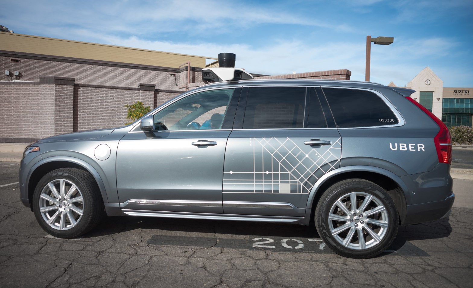
Camera perception is one of the most important building blocks in a self-driving car. If radar tells us that something is there and LiDAR helps estimate geometry, the camera gives the system something equally valuable: semantic understanding. A camera can tell us what a traffic light means, what a road sign says, where lane markings curve, whether an object is a pedestrian or a bicycle, and whether a patch of road is drivable or blocked.
That is why modern autonomous-driving and ADAS systems still rely heavily on cameras, even when they also use radar, LiDAR, ultrasound, and maps. In practice, the camera is often the sensor that gives the richest visual context to the perception stack.
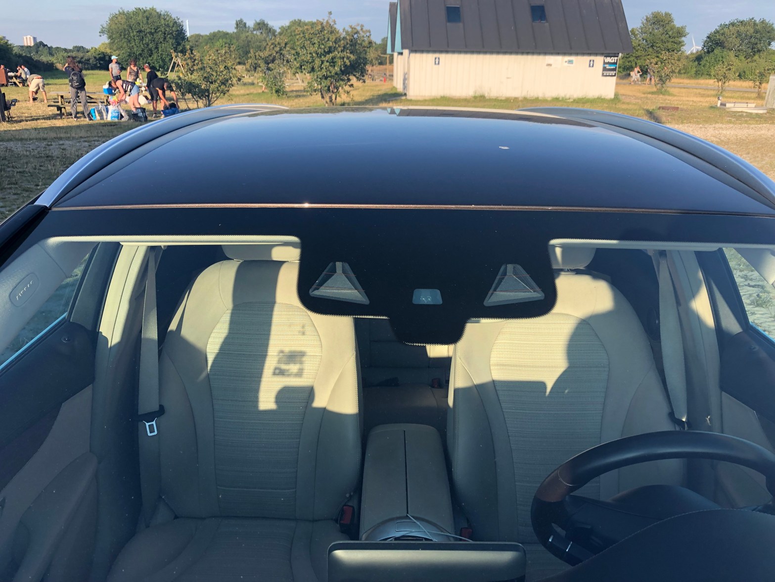
Camera modules mounted near the windshield are common in lane keeping, sign recognition, and driver-assistance systems. Source: Wikimedia Commons, Lane assist.jpg.
Why cameras matter so much
A self-driving vehicle does not just need distance. It needs meaning. The system must understand that a small red circle is a stop sign, that a green light means go, that a painted white line marks a lane boundary, and that a person at the curb may step into the road. These are tasks where cameras are especially strong because they capture texture, color, symbols, and shape in dense detail.
In real vehicles, cameras are used for tasks such as:
lane detection and lane geometry estimation
traffic-light and traffic-sign recognition
object detection and classification for cars, trucks, bikes, and pedestrians
free-space and drivable-area estimation
visual odometry, localization, and mapping
parking, surround view, blind-spot coverage, and driver monitoring
The practical advantage is cost and scalability. Cameras are relatively affordable, small, and information-rich, which is why many commercial ADAS platforms are camera-first or at least camera-centric. The limitation is that cameras are sensitive to bad lighting, glare, rain, fog, lens dirt, motion blur, and low texture. So the engineering question is not “camera or other sensors,” but rather “what should the camera do best, and what should be cross-checked by radar, LiDAR, or maps?”
How a camera sees the road
At the mathematical level, most automotive vision pipelines start with the pinhole camera model. A 3D point in the world is projected into a 2D pixel on the image plane. That sounds simple, but in practice you also need to account for lens distortion, focal length, principal point, camera pose, and synchronization with the rest of the vehicle.
The pinhole camera model is the foundation for projection, calibration, and many vision algorithms. Source: Wikimedia Commons, Pinhole camera model technical version.svg.
Three ideas matter here:
Intrinsics: focal lengths and principal point that describe how the lens and sensor map light into pixels.
Extrinsics: the rotation and translation between the camera and the vehicle frame or world frame.
Distortion: radial and tangential effects that bend straight lines unless the image is calibrated and rectified.
If calibration is poor, the whole stack becomes less trustworthy. Lane boundaries drift. Distance estimates become unstable. Multi-camera stitching looks wrong. That is why calibration is not a side issue; it is a core safety and reliability issue.
A small OpenCV-style example for undistortion looks like this:
This does not solve perception by itself, but it gives the rest of the pipeline a cleaner and more geometrically meaningful image.
The practical camera pipeline in a self-driving car
Once the image is captured, the perception system usually follows a pipeline similar to this:
Capture and synchronize. Frames must be time-aligned with other cameras, radar, IMU, wheel odometry, and vehicle state.
Calibrate and rectify. Remove distortion and align the image to the vehicle geometry.
Detect and segment. Use classical CV, deep learning, or both to extract lanes, drivable area, traffic lights, signs, and dynamic objects.
Track over time. A single frame is noisy. Multi-frame tracking stabilizes detections and estimates motion.
Estimate geometry. Recover depth from monocular cues, stereo disparity, multi-view triangulation, or fusion with radar/LiDAR.
Fuse and decide. Combine camera output with other sensors and planning logic to support motion decisions.
This is the difference between a demo and a production system. A demo may detect a lane in one image. A production system must maintain stable, low-latency, safety-aware perception under changing weather, different roads, oncoming headlights, and partial occlusion.
What the camera is especially good at
Cameras are the strongest sensor when the system needs semantic detail. Here are the most important examples.
1. Lane understanding
Lane perception is more than finding two white lines. A useful system must estimate lane boundaries, lane center, curvature, merges, splits, missing paint, shadows, and construction zones. In older pipelines, engineers used color thresholding, edge detection, perspective transforms, and Hough lines. In modern systems, deep learning often handles lane segmentation or direct lane representation, but the classical ideas still matter because they explain the geometry and help with debugging.
A simple lane-detection example showing how edge detection and line fitting can isolate lane candidates. Source: Wikimedia Commons, Lane Detection Example.jpg.
In practice, lane perception supports downstream tasks such as lane keeping, trajectory generation, highway navigation, and safety envelopes around the vehicle.
2. Traffic lights and signs
This is where cameras become indispensable. Radar cannot tell whether a light is red or green. LiDAR does not naturally read sign text or arrow direction. Cameras can. That makes them essential for semantic compliance with traffic rules.
A robust traffic-light stack must handle small objects at distance, occlusion, backlighting, LED flicker, and confusing urban scenes. A robust sign-recognition stack must classify signs correctly, but also decide whether a sign applies to the ego lane.
3. Object classification
Knowing that “something exists” is not enough. The planner needs to know whether that object is a pedestrian, cyclist, car, truck, cone, stroller, or road debris. Cameras provide the appearance cues that make this possible.
This is also where temporal reasoning matters. A pedestrian at the sidewalk is not the same as a pedestrian stepping into the crosswalk. The camera gives the appearance; tracking across frames gives intent clues.
4. Visual odometry and localization
Cameras are also useful for localization. By matching features across frames and across maps, the system can estimate motion and refine its position. This becomes even more powerful in stereo or surround-view configurations, or when fused with IMU and map information.
Monocular, stereo, and surround-view setups
Not all camera systems are the same.
Monocular camera: cheapest and simplest, strong for classification and lane understanding, weaker for absolute depth unless combined with motion or learned depth cues.
Stereo camera: adds geometric depth through disparity, especially useful at short and medium range.
Surround-view multi-camera: provides near-360-degree coverage for parking, blind spots, intersections, and urban driving.
Stereo vision estimates depth by measuring disparity between left and right images. Source: Wikimedia Commons, Stereovision.gif.
The key stereo idea is simple: a nearby object appears at different horizontal positions in the left and right image. That disparity can be converted to depth. In real systems, however, stereo only works well when calibration and rectification are correct, texture is sufficient, and weather or lighting does not destroy image quality.
Where cameras struggle
It is just as important to understand the limits of cameras.
Night and low light: semantic detail drops and noise rises.
Rain, fog, snow, glare: visibility degrades and the model sees less contrast.
Dirty or blocked lenses: perception can fail locally even if the rest of the system is healthy.
Motion blur and rolling shutter: fast motion distorts geometry.
Depth ambiguity: monocular vision is weak at absolute metric depth without additional assumptions or fusion.
That is why production systems rarely trust a camera alone for all situations. Camera-first makes sense for semantics and scale, but sensor fusion still matters for robustness.
Why camera-first still makes sense
Even with those weaknesses, cameras remain central because they match several practical engineering goals at once:
they capture dense visual information
they are cheaper and easier to scale than high-end active sensors
they support the semantic tasks that every road-legal system must solve
they fit both ADAS and higher-autonomy stacks
That is why many commercial systems use a camera-first or camera-centric architecture, then add radar, LiDAR, maps, and driver monitoring where the safety case demands it.
A practical engineering checklist
If you are building or evaluating a camera-based perception stack, these are the questions that matter most:
How stable is calibration over time, temperature, vibration, and mounting changes?
What happens under glare, nighttime, rain, and lens contamination?
How much latency exists from image capture to decision output?
Which tasks are vision-only, and which require fusion?
How is uncertainty represented and passed to planning?
Does the system fail gracefully when the image quality drops?
Those questions usually separate a classroom demo from an automotive-grade perception module.
Conclusion
The camera is not just a passive eye on a self-driving car. It is the main source of semantic road understanding. It tells the system what the world means, not just where something is. That makes cameras essential for lane understanding, traffic-light recognition, sign reading, object classification, localization, and many driver-assistance functions.
At the same time, good camera perception depends on careful calibration, stable geometry, robust learning models, temporal tracking, and realistic handling of bad-weather and low-light failures. In other words, the power of cameras in autonomous driving is real, but it only becomes useful when the full engineering pipeline around the camera is strong.
Self-driving systems are often explained as separate modules: localization, perception, prediction, planning, and control. That modular view is useful, but it can also be misleading. A real autonomous-driving stack does not succeed because one block is excellent in isolation. It succeeds because the blocks exchange the right information, at the right time, with the right assumptions.
That is what system integration really means. It is the engineering discipline of connecting sensing, localization, maps, planning, control, and vehicle interfaces into one coherent pipeline that can operate safely under real-world timing and uncertainty constraints.
Why integration matters more than slideware
A strong perception model is not enough if localization drifts. A good planner is not enough if control cannot follow the trajectory. A precise controller is not enough if the vehicle interface delays commands or clips them unexpectedly. In practice, many failures appear at the boundaries between modules rather than inside a single algorithm.
That is why mature autonomous-driving projects place so much emphasis on interfaces, diagnostics, synchronization, fallback behavior, and system architecture.
The major building blocks
A practical self-driving stack usually contains these major layers:
Localization: estimate current pose, velocity, and acceleration.
Perception: detect lanes, objects, traffic lights, free space, and obstacles.
Prediction: estimate how other agents may move next.
Planning: choose a safe route, path, and trajectory.
Control: convert the planned trajectory into steering, acceleration, and braking commands.
Vehicle interface: deliver those commands safely to the actual platform.
These blocks are familiar, but the real work is in their coordination.
How information flows through the system
A useful integrated stack behaves like a pipeline with feedback, not like a row of isolated boxes.
sensors
    -> localization
    -> perception
    -> prediction
    -> planning
    -> control
    -> vehicle interface

diagnostics and state feedback
    -> monitor health, uncertainty, delays, and fallback modes
Autoware’s architecture documents make this dependency clear. Planning depends on information from localization, perception, and maps. Control depends on the reference trajectory from planning. Localization itself may depend on LiDAR maps, IMU data, and vehicle velocity. If any upstream information is stale or unstable, the downstream behavior degrades.
Localization is not just a coordinate estimate
In an integrated system, localization must provide more than a rough pose. It must provide:
pose in the map frame
velocity and acceleration estimates
covariance or confidence information
timestamps that align with the rest of the pipeline
That information is consumed directly by planning and control. If localization lags behind reality or reports unstable motion, planning may generate a trajectory that is already outdated.
Perception must produce planning-ready outputs
Perception often gets too much attention as a standalone benchmark problem. But in a vehicle stack, the most important question is not whether perception is impressive in a paper. It is whether it produces the exact outputs planning needs.
For example, planning may need:
detected objects with stable tracks
obstacle information for emergency stopping
occupancy information for occluded regions
traffic-light recognition tied to the relevant route
This is one reason Autoware’s documentation describes planning inputs very carefully: the planner relies on structured, timely, route-relevant environment information, not on generic detections alone.
Planning and control are tightly linked
Planning produces a trajectory, but that trajectory is only useful if control can execute it. Control modules need trajectories that are smooth, physically feasible, and consistent with the actual vehicle model. If the planner outputs unrealistic curvature or aggressive accelerations, the controller either fails or compensates in ways that create instability.
Autoware’s control design documents highlight exactly this relationship: control follows the reference trajectory from planning and converts it into target steering, speed, and acceleration commands. That is a clean architectural separation, but it still requires the planner and controller to agree on timing, kinematics, and limits.
What system integration usually includes
In practice, system integration is not only about software wiring. It includes:
message contracts and interface definitions
coordinate frames and transforms
sensor synchronization
health monitoring and diagnostics
latency budgeting
fallback and degradation strategies
vehicle-specific adaptation layers
That last point matters. A generic autonomy stack often outputs abstract commands such as target speed, acceleration, and steering angle. A vehicle-specific adapter then maps those commands to the actual hardware interface. This is another place where integration quality matters enormously.
Common integration failures
Some of the most important failures in autonomous systems are integration failures, not algorithmic failures:
timestamps from different sensors do not align
map and vehicle frames are inconsistent
perception outputs are too noisy for planning
control receives trajectories it cannot track smoothly
diagnostics do not catch degraded modules quickly enough
vehicle adapters change behavior relative to what higher layers expect
These problems can make a technically strong stack behave unpredictably in the field.
What a good integrated stack looks like
A well-integrated self-driving stack tends to have these qualities:
clear interfaces between modules
consistent coordinate frames and timing
explicit uncertainty and diagnostics
modular components that can still be validated end-to-end
graceful degradation when one sensor or module weakens
In other words, good system integration does not remove modularity. It makes modularity usable in a real vehicle.
A practical checklist
If I were reviewing a self-driving integration effort, I would ask:
Which modules define the system time base and synchronization policy?
How are localization confidence and perception uncertainty passed downstream?
What happens when planning receives stale or inconsistent inputs?
Can control reject trajectories it cannot safely follow?
How is the vehicle interface validated against actual hardware response?
What diagnostics trigger fallback or minimal risk behavior?
Those questions often reveal the real maturity of the stack faster than demo footage does.
Conclusion
System integration is what turns separate autonomy modules into an actual self-driving system. Localization, perception, planning, control, and the vehicle interface must agree not only on data format, but also on timing, confidence, physical limits, and safety behavior. That is why system integration is not a final polish step. It is one of the core engineering problems in autonomous driving.
Autonomous systems do not rely on a single technology. They work because several layers of perception support each other. Computer vision extracts visual structure, deep learning helps recognize patterns and objects, and sensors provide the raw measurements needed to understand the environment.
Computer Vision vs Deep Learning
These two ideas are related, but not identical. Traditional computer vision focuses on geometry, edges, features, transformations, calibration, and image processing. Deep learning focuses on learning complex patterns from data, often through neural networks.
In practice, modern systems use both. Geometry still matters, and learned perception has become essential.
Why Sensors Matter
A camera gives rich visual data, but no single sensor is enough in all conditions. Real autonomous systems often combine:
cameras for semantics and rich scene information,
LiDAR for geometry and depth structure,
radar for robustness in difficult weather,
IMU and odometry for short-term motion tracking.
A Practical Pipeline
A perception stack in an autonomous vehicle may look like this:
Cameras capture road scenes.
Deep models detect lanes, vehicles, pedestrians, and signs.
LiDAR or radar improves distance estimation and object consistency.
Sensor fusion tracks objects over time.
The planning stack uses this interpreted scene to make decisions.
Where Traditional Vision Still Helps
camera calibration,
stereo depth estimation,
visual odometry,
image rectification,
pose estimation and geometry-based reasoning.
Where Deep Learning Adds Value
object detection,
semantic segmentation,
lane understanding,
driver or pedestrian behavior cues,
end-to-end learned scene interpretation.
Final Thoughts
The strongest autonomous systems are not built by choosing between classical computer vision and deep learning. They are built by using the right combination of sensing, geometry, learning, and engineering discipline for the task at hand.
Kubernetes, often shortened to K8s, is a container orchestration platform designed to run and manage applications across clusters of machines. It became popular because running one container is easy, but running many services reliably in production is much harder.
What Kubernetes Actually Solves
At a high level, Kubernetes helps teams deploy applications consistently, scale them, recover from failures, and expose them through stable networking. It gives a standard control model for distributed applications.
Important Core Objects
Pods
A pod is the smallest deployable unit in Kubernetes. It usually contains one application container plus any closely related helper containers.
Deployments
Deployments manage the desired number of pod replicas and support rolling updates.
Services
Services provide stable access to a group of pods even when pod IPs change.
ConfigMaps and Secrets
These help separate configuration and sensitive values from the container image.
Ingress
Ingress provides HTTP routing so external users can reach services inside the cluster.
A Small Real-World Example
Imagine a web application with three parts:
a frontend service,
a backend API,
and a worker processing background jobs.
With Kubernetes, you can package each one as a container, run them as deployments, expose the frontend and API with services, and scale the worker independently when background load increases.
It helps large teams manage many services consistently.
Why Kubernetes Can Be Painful
It adds operational complexity.
Debugging networking and configuration issues can be time-consuming.
Not every small project needs cluster-level orchestration.
Kubernetes is powerful, but it is not a badge of maturity by itself. The right question is whether its operational model matches your scale and team capability.
Final Thoughts
Kubernetes is best understood as an operational platform, not just a trendy technology. If your system already needs scaling, resilience, and service coordination, Kubernetes can be a strong solution. If not, simpler deployment models may be better.
Infrastructure as Code, usually shortened to IaC, is the practice of managing infrastructure through code instead of manual clicks in a cloud console. Instead of creating servers, networks, IAM roles, and storage by hand, teams define them in version-controlled files and apply them consistently across environments.
Why Infrastructure as Code matters
Manual infrastructure changes are slow, difficult to review, and easy to forget. IaC solves this by making infrastructure reproducible. A team can create the same environment for development, staging, and production with far less drift.
Infrastructure becomes reviewable through pull requests
Changes can be repeated safely in multiple environments
Disaster recovery becomes faster because environments can be rebuilt
Documentation improves because the code itself describes the system
Popular Infrastructure as Code tools
Different tools solve different layers of the problem:
Terraform for cloud resources such as VPCs, EC2, IAM, S3, and Kubernetes clusters
Ansible for configuration and software setup on existing hosts
CloudFormation if you are heavily invested in AWS-native tooling
Helm for packaging and deploying applications on Kubernetes
Even this tiny example shows the core idea: infrastructure is declared, reviewed, and applied in a consistent way.
Best practices
Keep state management secure and backed up
Separate environments clearly
Review all IaC changes via pull requests
Use modules or reusable components to avoid duplication
Never hardcode secrets in IaC files
Final thoughts
Infrastructure as Code is not only about automation. It is about making infrastructure predictable, testable, and maintainable. Teams that adopt IaC well usually move faster and recover from mistakes more confidently.
Cloud technology is the delivery of computing resources over the internet. Instead of buying and maintaining every server yourself, you use services such as virtual machines, storage, managed databases, and serverless functions on demand.
The three common service models
IaaS gives you infrastructure such as virtual machines, networks, and disks
PaaS gives you a managed platform for deploying applications
SaaS gives you a finished software product delivered over the web
Imagine a web application with three parts: a frontend, a backend API, and a database. In a cloud setup, you might host the frontend on object storage + CDN, run the API in containers, and use a managed PostgreSQL service for the database. That architecture reduces the amount of infrastructure you must maintain yourself.
Cloud is not magic
The cloud makes many things easier, but it does not remove architecture decisions, security concerns, or cost management. Poor resource design can still lead to outages, expensive bills, or performance issues.
Final thoughts
Cloud technology matters because it changes how quickly teams can build and scale systems. Understanding compute, networking, storage, identity, and observability in the cloud is a core skill for modern software and DevOps engineers.


