Kubernetes, often shortened to K8s, is a container orchestration platform designed to run and manage applications across clusters of machines. It became popular because running one container is easy, but running many services reliably in production is much harder.
What Kubernetes Actually Solves
At a high level, Kubernetes helps teams deploy applications consistently, scale them, recover from failures, and expose them through stable networking. It gives a standard control model for distributed applications.
Important Core Objects
Pods
A pod is the smallest deployable unit in Kubernetes. It usually contains one application container plus any closely related helper containers.
Deployments
Deployments manage the desired number of pod replicas and support rolling updates.
Services
Services provide stable access to a group of pods even when pod IPs change.
ConfigMaps and Secrets
These help separate configuration and sensitive values from the container image.
Ingress
Ingress provides HTTP routing so external users can reach services inside the cluster.
A Small Real-World Example
Imagine a web application with three parts:
a frontend service,
a backend API,
and a worker processing background jobs.
With Kubernetes, you can package each one as a container, run them as deployments, expose the frontend and API with services, and scale the worker independently when background load increases.
It helps large teams manage many services consistently.
Why Kubernetes Can Be Painful
It adds operational complexity.
Debugging networking and configuration issues can be time-consuming.
Not every small project needs cluster-level orchestration.
Kubernetes is powerful, but it is not a badge of maturity by itself. The right question is whether its operational model matches your scale and team capability.
Final Thoughts
Kubernetes is best understood as an operational platform, not just a trendy technology. If your system already needs scaling, resilience, and service coordination, Kubernetes can be a strong solution. If not, simpler deployment models may be better.
Infrastructure as Code, usually shortened to IaC, is the practice of managing infrastructure through code instead of manual clicks in a cloud console. Instead of creating servers, networks, IAM roles, and storage by hand, teams define them in version-controlled files and apply them consistently across environments.
Why Infrastructure as Code matters
Manual infrastructure changes are slow, difficult to review, and easy to forget. IaC solves this by making infrastructure reproducible. A team can create the same environment for development, staging, and production with far less drift.
Infrastructure becomes reviewable through pull requests
Changes can be repeated safely in multiple environments
Disaster recovery becomes faster because environments can be rebuilt
Documentation improves because the code itself describes the system
Popular Infrastructure as Code tools
Different tools solve different layers of the problem:
Terraform for cloud resources such as VPCs, EC2, IAM, S3, and Kubernetes clusters
Ansible for configuration and software setup on existing hosts
CloudFormation if you are heavily invested in AWS-native tooling
Helm for packaging and deploying applications on Kubernetes
Even this tiny example shows the core idea: infrastructure is declared, reviewed, and applied in a consistent way.
Best practices
Keep state management secure and backed up
Separate environments clearly
Review all IaC changes via pull requests
Use modules or reusable components to avoid duplication
Never hardcode secrets in IaC files
Final thoughts
Infrastructure as Code is not only about automation. It is about making infrastructure predictable, testable, and maintainable. Teams that adopt IaC well usually move faster and recover from mistakes more confidently.
Cloud technology is the delivery of computing resources over the internet. Instead of buying and maintaining every server yourself, you use services such as virtual machines, storage, managed databases, and serverless functions on demand.
The three common service models
IaaS gives you infrastructure such as virtual machines, networks, and disks
PaaS gives you a managed platform for deploying applications
SaaS gives you a finished software product delivered over the web
Imagine a web application with three parts: a frontend, a backend API, and a database. In a cloud setup, you might host the frontend on object storage + CDN, run the API in containers, and use a managed PostgreSQL service for the database. That architecture reduces the amount of infrastructure you must maintain yourself.
Cloud is not magic
The cloud makes many things easier, but it does not remove architecture decisions, security concerns, or cost management. Poor resource design can still lead to outages, expensive bills, or performance issues.
Final thoughts
Cloud technology matters because it changes how quickly teams can build and scale systems. Understanding compute, networking, storage, identity, and observability in the cloud is a core skill for modern software and DevOps engineers.
Google Cloud Platform, or GCP, is one of the major public cloud providers used to build, deploy, and operate modern software systems. In practice, GCP is not one tool but a collection of services for compute, storage, networking, security, data, and machine learning.
Why GCP Matters
Cloud platforms became important because teams needed faster infrastructure delivery, better scalability, and more reliable operations. Instead of buying and managing physical hardware for every project, engineers can provision resources on demand and pay only for what they use.
GCP is especially attractive for teams that care about strong data tooling, Kubernetes, global infrastructure, and integration with modern developer workflows.
Core GCP Services
Compute Engine
Virtual machines for workloads that need direct operating system control. This is often the easiest place to start if you want cloud flexibility without changing application architecture too much.
Google Kubernetes Engine (GKE)
Managed Kubernetes for containerized applications. GKE reduces operational work around control plane management and makes it easier to run microservices at scale.
Cloud Storage
Object storage for backups, logs, artifacts, static assets, and analytics pipelines.
Cloud SQL and Firestore
Managed databases for transactional applications and document-style data models.
BigQuery
A powerful analytics warehouse for large-scale data querying. This is one of the most recognized strengths of GCP.
A Practical Architecture Example
Consider a small SaaS platform:
The frontend is hosted behind a load balancer.
The backend API runs on GKE or Compute Engine.
Images and static assets are stored in Cloud Storage.
Application data lives in Cloud SQL.
Logs and metrics are exported to monitoring dashboards.
Analytics queries run in BigQuery.
This kind of architecture shows why cloud platforms are valuable: services are separated, scalable, and easier to operate than a manually managed monolith on one server.
What Engineers Should Understand Early
IAM: permission design matters from day one.
Networking: VPCs, subnets, firewalls, and ingress rules affect both security and availability.
Cost awareness: managed services are convenient, but convenience without monitoring can become expensive.
Observability: logs, metrics, and alerts are not optional in cloud systems.
When GCP Is a Good Fit
teams already using containers and Kubernetes,
data-heavy products needing analytics pipelines,
engineering organizations that want managed infrastructure with strong APIs,
projects that benefit from global services and quick scaling.
Final Thoughts
GCP becomes much easier to understand when you stop treating it as a long list of services and start treating it as a toolbox for building systems. The real skill is not memorizing product names. The real skill is understanding which managed service solves which operational problem.
The Iris dataset is one of the best beginner examples for understanding the perceptron. It is small, well known, and easy to visualize. That makes it a practical way to see how a linear classifier learns from real feature values rather than only from toy Boolean inputs.
In this article, we use the Iris dataset to train a perceptron in Python and explain what the result actually teaches. The goal is not only to show code. The goal is to understand why this dataset works well as a first perceptron example.
What you will learn
why the Iris dataset is a good starting point
how to prepare a binary classification task for the perceptron
how the training loop works on real feature data
what to expect from the result and where the model starts to struggle
Why the Iris dataset is useful here
Scikit-learn’s Iris example describes the dataset as 150 samples with four features across three iris species. For a beginner, that is perfect because the data is simple enough to inspect while still being real tabular classification data.
A common first step is to simplify the task into a binary classification problem. For example, you can choose two classes and focus on two features such as petal length and petal width. That keeps the geometry easy to visualize and matches the perceptron’s linear nature.
Preparing the data
from sklearn.datasets import load_iris
import numpy as np

iris = load_iris()
X = iris.data[:, [2, 3]]  # petal length and petal width
y = iris.target

# keep only two classes for a binary perceptron example
mask = y < 2
X = X[mask]
y = y[mask]
This transforms the classic three-class dataset into a much cleaner binary problem that a single perceptron can handle more naturally.
Training a perceptron
You can train either a scratch implementation or the scikit-learn version. The scratch route is best for intuition. The scikit-learn route is best when you want a fast verified baseline.
from sklearn.linear_model import Perceptron

model = Perceptron(max_iter=1000, tol=1e-3, random_state=42)
model.fit(X, y)
predictions = model.predict(X)
Scikit-learn’s documentation notes that its perceptron classifier is implemented as a wrapper around `SGDClassifier` with a perceptron loss and constant learning rate. That is useful context because it shows the historical model inside a modern linear-learning framework.
What the result means
If you choose two well-separated classes and helpful features, the perceptron often performs very well on this simplified Iris task. That result should not be read as “the perceptron solves general machine learning.” It should be read more carefully:
the problem has been simplified into a binary task
the selected features support a fairly clean separation
the perceptron succeeds because the geometry is favorable
This is exactly why Iris is a teaching dataset. It helps you see when a linear classifier is a good fit.
What to inspect during training
When working through this example, pay attention to:
which two classes you selected
which two features you used
whether the points look roughly linearly separable
how stable the predictions become after training
If you change the task to something less separable, the perceptron can struggle. That is not surprising. It is the same structural limitation discussed in Why perceptrons fail on xor.
Why this example is worth keeping on the site
The Iris article is a strong supporting piece in the Perceptron cluster because it connects theory to data. The pillar article Perceptron explained for beginners teaches the concept. This article shows the concept on a familiar dataset. Together, they make the topic much easier to trust and understand.
Common mistakes or limitations
using all three Iris classes and expecting a simple binary explanation
not checking whether the chosen features are linearly separable enough
treating a clean toy result as proof that the model is broadly strong
confusing dataset convenience with real-world robustness
Key takeaways
The Iris dataset is a strong beginner example for the perceptron because it is small and interpretable.
A binary subset with suitable features fits the perceptron especially well.
The example teaches when a linear classifier works, not that it works everywhere.
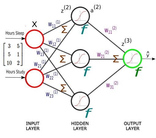
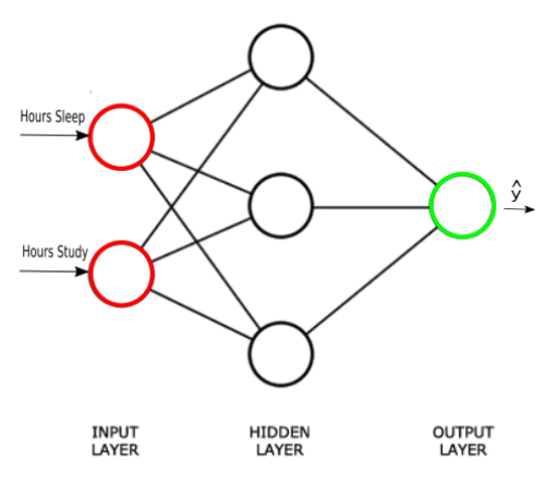
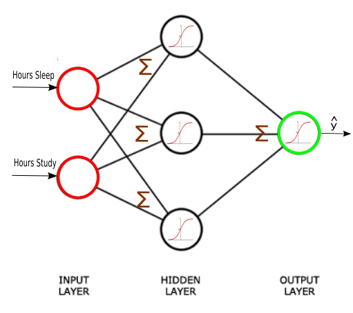
The Neural network structure is: one, input layer, one output layer, and layers between are hidden layer.
Introduction
An Artificial Neural Network (ANN) is an interconnected group of nodes, similar to the our brain network.
Here, we have three layers, and each circular node represents a neuron and a line represents a connection from the output of one neuron to the input of another.
The first layer has input neurons which send data via synapses to the second layer of neurons, and then via more synapses to the third layer of output neurons.
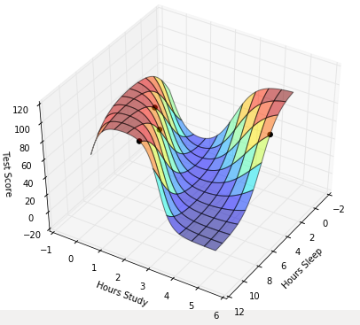
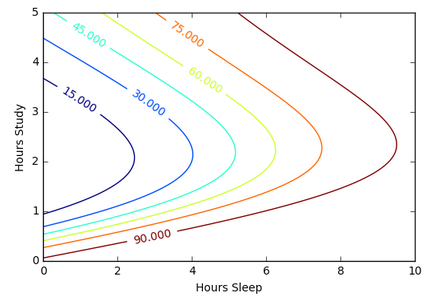
Suppose we want to predict our test score based on how many hours we sleep and how many hours we study the night before.
In other words, we want to predict output value yy which are scores for a given set of input values XX which are hours of (sleep, study).
XX (sleep, study)
y (test score)
(3,5)
75
(5,1)
82
(10,2)
93
(8,3)
?
In our machine learning approach, we’ll use the python to store our data in 2-dimensional numpy arrays.
We’ll use the data to train a model to predict how we will do on our next test.
This is a supervised regression problem.
It’s supervised because our examples have outputs(yy).
It’s a regression because we’re predicting the test score, which is a continuous output.
If we we’re predicting the grade (A,B, etc.), however, this is going to be a classification problem but not a regression problem.
We may want to scale our data so that the result should be in [0,1].
Now we can start building our Neural Network.
We know our network must have 2 inputs(XX) and 1 output(yy).
We’ll call our output y^y^, because it’s an estimate of yy.
Any layer between our input and output layer is called a hidden layer. Here, we’re going to use just one hidden layer with 3 neurons.
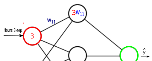
Neurons synapses
As explained in the earlier section, circles represent neurons and lines represent synapses.
Synapses have a really simple job.
They take a value from their input, multiply it by a specific weight, and output the result. In other words, the synapses store parameters called “weights” which are used to manipulate the data.
Neurons are a little more complicated.
Neurons’ job is to add together the outputs of all their synapses, and then apply an activation function.
Certain activation functions allow neural nets to model complex non-linear patterns.
For our neural network, we’re going to use sigmoid activation functions.
This will be a very brief tutorial on Docker: we’ll take a “nginx” docker image and build a simple web server on Docker container. In that process, we can get a quick taste of how Docker is working.
We’ll learn:
How to get an official image.
How to use the files on host machine from our container.
How to copy the files from our host to the container.
How to make our own image – in this tutorial, we’ll make a Dockerfile with a page for render.
Getting Nginx official docker image
To create an instance of Nginx in a Docker container, we need to search for and pull the Nginx official image from Docker Hub. Use the following command to launch an instance of Nginx running in a container and using the default configuration:
$ docker container run --name my-nginx-1 -P -d nginx
f0cea39a8bc38b38613a3a4abe948d0d1b055eefe86d026a56c783cfe0141610
The command creates a container named “my-nginx-1” based on the Nginx image and runs it in “detached” mode, meaning the container is started and stays running until stopped but does not listen to the command line. We will talk about this later how to interact with the container.
The Nginx image exposes ports 80 and 443 in the container and the -P option tells Docker to map those ports to ports on the Docker host that are randomly selected from the range between 49153 and 65535.
We do this because if we create multiple Nginx containers on the same Docker host, we may induce conflicts on ports 80 and 443. The port mappings are dynamic and are set each time the container is started or restarted.
If we want the port mappings to be static, set them manually with the -p option. The long form of the “Container Id” will be returned.
We can run docker ps to verify that the container was created and is running, and to see the port mappings:
$ docker container ps
CONTAINER ID IMAGE COMMAND                 CREATED       STATUS       PORTS                                        NAMES
f0cea39a8bc3 nginx "nginx -g 'daemon off"  5 minutes ago Up 5 minutes 0.0.0.0:32769->80/tcp   my-nginx-1
We can verify that Nginx is running by making an HTTP request to port 32769 (reported in the output from the preceding command as the port on the Docker host that is mapped to port 80 in the container), the default Nginx welcome page appears:
$ docker container stop f0cea39a8bc3
f0cea39a8bc3

$ docker container ps
CONTAINER ID        IMAGE               COMMAND             CREATED             STATUS              PORTS               NAMES

$ docker container rm f0cea39a8bc3
If we want to map the container’s port 80 to a specific port of the host, we can use -p with host_port:docker_port:
$ docker container run --name my-nginx-1 -p8088:80 -d nginx
bd39cc4ed6dbba92e85437b0ab595e92c5ca2e4a87ee3e724a0cf04aa9726044

$ docker container ps
CONTAINER ID  IMAGE  COMMAND                 CREATED         STATUS         PORTS                  NAMES
bd39cc4ed6db  nginx  "nginx -g 'daemon of…"  18 seconds ago  Up 18 seconds  0.0.0.0:8088->80/tcp   my-nginx-1
More work on the Nginx Docker Container
Now that we have a working Nginx Docker container, how do we manage the content and the configuration? What about logging?
It is common to have SSH access to Nginx instances, but Docker containers are generally intended to be for a single purpose (in this case running Nginx) so the Nginx image does not have OpenSSH installed and for normal operations there is no need to get shell access directly to the Nginx container. We will use other methods supported by Docker rather than using SSH.
Keep the Content and Configuration on the Docker Host
When the container is created, we can tell Docker to mount a local directory on the Docker host to a directory in the container.
The Nginx image uses the default Nginx configuration, so the root directory for the container is /usr/share/nginx/html. If the content on the Docker host is in the local directory /tmp/nginx/html, we run the command:
$ docker container run --name my-nginx-2 \
-v /tmp/nginx/html:/usr/share/nginx/html:ro -P -d nginx

$ docker container ps
CONTAINER ID  IMAGE  COMMAND                CREATED       STATUS       PORTS                   NAMES
35a4c74ff073  nginx  "nginx -g 'daemon off" 7 seconds ago Up 2 seconds 0.0.0.0:32770->80/tcp   my-nginx-2
Now any change made to the files in the local directory, /tmp/nginx/html on the Docker host are reflected in the directories /usr/share/nginx/html in the container. The :ro option causes these directors to be read only inside the container.
Copying files from the Docker host
Rather than using the files that kept in the host machine, another option is to have Docker copy the content and configuration files from a local directory on the Docker host when a container is created.
Once a container is created, the files are maintained by creating a new container when the files change or by modifying the files in the container.
A simple way to copy the files is to create a Dockerfile to generate a new Docker image, based on the Nginx image from Docker Hub. When copying files in the Dockerfile, the path to the local directory is relative to the build context where the Dockerfile is located. For this example, the content is in the MyFiles directory under the same directory as the Dockerfile.
Here is the Dockerfile:
FROM nginx
COPY MyFiles /usr/share/nginx/html
We can then create our own Nginx image by running the following command from the directory where the Dockerfile is located:
Note the period (“.”) at the end of the command. This tells Docker that the build context is the current directory. The build context contains the Dockerfile and the directories to be copied.
Now we can create a container using the image by running the command:
$ docker container run --name my-nginx-3 -P -d my-nginx-image-1
150fe5eddb31acde7dd432bed73f8daba2a7eec3760eb272cb64bfdd2809152d

$ docker container ps
CONTAINER ID  IMAGE             COMMAND                  CREATED        STATUS        PORTS                   NAMES
150fe5eddb31  my-nginx-image-1  "nginx -g 'daemon of…"   7 seconds ago  Up 7 seconds  0.0.0.0:32772->80/tcp   my-nginx-3
Editing (Sharing) files in Docker container : volumes
Actually, the volume of Docker belongs to an advanced level. So, in this section, we only touch the topic briefly.
As we know, we are not able to get SSH access to the Nginx container, so if we want to edit the container files directly we can use a helper container that has shell access.
In order for the helper container to have access to the files, we must create a new image that has the proper volumes specified for the image.
Assuming we want to copy the files as in the example above, while also specifying volumes for the content and configuration files, we use the following Dockerfile:
FROM nginx
COPY content /usr/share/nginx/html
VOLUME /myVolume-1
We then create the new Nginx image (my-nginx-image-2) by running the following command:
Now we create an Nginx container (my-nginx-4) using the image by running the command:
$ docker container run --name my-nginx-4 -P -d my-nginx-image-2
8c84cf08dc08a0b00bd04c9b7047ff65f1ec5c910aa6b096a743b18652e128f9
We then start a helper container with a shell and access the content and configuration directories of the Nginx container we created in the previous example by running the command:
This creates an interactive container named my-nginx-4-with-volume that runs in the foreground with a persistent standard input (-i) and a tty (-t) and mounts all the volumes defined in the container my-nginx-4 as local directories in the my-nginx-4-with-volume container.
After the container is created, it runs the bash shell, which presents a shell prompt for the container that we can use to modify the files as needed.
Now, we can check the volume has been mounted:
root@64052ed5e1b3:/# ls
bin  boot  dev	etc  home  lib	lib64  media  mnt  myVolume-1  opt  proc  root	run  sbin  srv	sys  tmp  usr  var
root@64052ed5e1b3:/#
To check the volume on local machine we can go to /var/lib/docker/volumes. On Mac system, we need to take an additional step to:
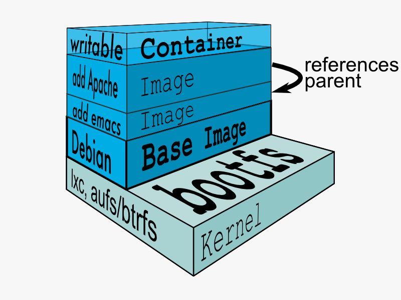
The problem with Virtual Machines built using VirtualBox or VMWare is that we have to run entire OS for every VM. That’s where Docker comes in. Docker virtualizes on top of one OS so that we can run Linux using technology known as LinuX Containers (LXC). LXC combines cgroups and namespace support to provide an isolated environment for applications. Docker can also use LXC as one of its execution drivers, enabling image management and providing deployment services.
Docker allows us to run applications inside containers. Running an application inside a container takes a single command: docker run.
Docker Registry – Repositories of Docker Images
We need to have a disk image to make the virtualization work. The disk image represents the system we’re running on and they are the basis of containers.
Docker registry is a registry of already existing images that we can use to run and create containerized applications.
There are lots of communities and works already been done to build the system. Docker company supports and maintains its registry and the community around it.
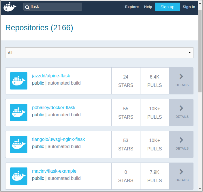
We can search images within the registry hub, for example, the sample picture is the result from searching “flask”.
Docker search
The Docker search command allows us to go and look at the registry in search for the images that we want.
$ docker search --help

Usage: docker search [OPTIONS] TERM

Search the Docker Hub for images

  --automated=false    Only show automated builds
  --no-trunc=false     Don't truncate output
  -s, --stars=0        Only displays with at least x stars
If we do the same search, Jenkins, we get exactly the same result as we got from the web:
$ docker search ubuntu
NAME                      DESCRIPTION                                    STARS  OFFICIAL   AUTOMATED
ubuntu                    Ubuntu is a Debian-based Linux operating s...  5969     [OK]
rastasheep/ubuntu-sshd    Dockerized SSH service, built on top of of...  83                   [OK]
ubuntu-upstart            Upstart is an event-based replacement for ...  71       [OK]
ubuntu-debootstrap        debootstrap --variant=minbase --components...  30       [OK]
torusware/speedus-ubuntu  Always updated official Ubuntu docker imag...  27                   [OK]
nuagebec/ubuntu           Simple always updated Ubuntu docker images...  20                   [OK]
...
We got too many outputs, so we need to filter it out items with more than 10 stars:
$ docker search --filter=stars=20 ubuntu
NAME                      DESCRIPTION                                    STARS   OFFICIAL   AUTOMATED
ubuntu                    Ubuntu is a Debian-based Linux operating s...  5969      [OK]
rastasheep/ubuntu-sshd    Dockerized SSH service, built on top of of...  83                   [OK]
ubuntu-upstart            Upstart is an event-based replacement for ...  71        [OK]
ubuntu-debootstrap        debootstrap --variant=minbase --components...  30        [OK]
torusware/speedus-ubuntu  Always updated official Ubuntu docker imag...  27                   [OK]
nuagebec/ubuntu           Simple always updated Ubuntu docker images...  20                   [OK]
Docker pull
Once we found the image we like to use it, we can use Docker’s pull command:
$ docker pull --help

Usage:	docker pull [OPTIONS] NAME[:TAG|@DIGEST]

Pull an image or a repository from a registry

Options:
  -a, --all-tags                Download all tagged images in the repository
      --disable-content-trust   Skip image verification (default true)
      --help                    Print usage
The pull command will go up to the web site and grab the image and download it to our local machine.
The pull command without any tag will download all Ubuntu images though I’ve already done it. To see what Docker images are available on our machine, we use docker images:
$ docker images
REPOSITORY          TAG                 IMAGE ID            CREATED             VIRTUAL SIZE
ubuntu              latest              5506de2b643b        4 weeks ago         199.3 MB
So, the output indicates only one image is currently on my local machine. We also see the image has a TAG inside of it.
As we can see from the command below, docker pull centos:latest, we can also be more specific, and download only the version we need. In Docker, versions are marked with tags.
$ docker pull centos:latest
centos:latest: The image you are pulling has been verified
5b12ef8fd570: Pull complete
ae0c2d0bdc10: Pull complete
511136ea3c5a: Already exists
Status: Downloaded newer image for centos:latest
Here is the images on our local machine.
$ docker images
REPOSITORY          TAG                 IMAGE ID            CREATED             VIRTUAL SIZE
centos              latest              ae0c2d0bdc10        2 weeks ago         224 MB
ubuntu              latest              5506de2b643b        4 weeks ago         199.3 MB
The command, docker images, returns the following columns:
REPOSITORY: The name of the repository, which in this case is “ubuntu”.
TAG: Tags represent a specific set point in the repositories’ commit history. As we can see from the list, we’ve pulled down different versions of linux. Each of these versions is tagged with a version number, a name, and there’s even a special tag called “latest” which represents the latest version.
IMAGE ID: This is like the primary key for the image. Sometimes, such as when we commit a container without specifying a name or tag, the repository or the tag is <NONE>, but we can always refer to a specific image or container using its ID.
CREATED: The date the repository was created, as opposed to when it was pulled. This can help us assess how “fresh” a particular build is. Docker appears to update their master images on a fairly frequent basis.
VIRTUAL SIZE: The size of the image.
Docker run
Now we have images on our local machine. What do we do with them? This is where docker run command comes in.
$ docker run  --help

Usage: docker run [OPTIONS] IMAGE [COMMAND] [ARG...]

Run a command in a new container

  -a, --attach=[]            Attach to STDIN, STDOUT or STDERR.
  --add-host=[]              Add a custom host-to-IP mapping (host:ip)
  -c, --cpu-shares=0         CPU shares (relative weight)
  --cap-add=[]               Add Linux capabilities
  --cap-drop=[]              Drop Linux capabilities
  --cidfile=""               Write the container ID to the file
  --cpuset=""                CPUs in which to allow execution (0-3, 0,1)
  -d, --detach=false         Detached mode: run the container in the background and print the new container ID
  --device=[]                Add a host device to the container (e.g. --device=/dev/sdc:/dev/xvdc)
  --dns=[]                   Set custom DNS servers
  --dns-search=[]            Set custom DNS search domains
  -e, --env=[]               Set environment variables
  --entrypoint=""            Overwrite the default ENTRYPOINT of the image
  --env-file=[]              Read in a line delimited file of environment variables
  --expose=[]                Expose a port from the container without publishing it to your host
  -h, --hostname=""          Container host name
  -i, --interactive=false    Keep STDIN open even if not attached
  --link=[]                  Add link to another container in the form of name:alias
  --lxc-conf=[]              (lxc exec-driver only) Add custom lxc options --lxc-conf="lxc.cgroup.cpuset.cpus = 0,1"
  -m, --memory=""            Memory limit (format: <number><optional unit>, where unit = b, k, m or g)
  --name=""                  Assign a name to the container
  --net="bridge"             Set the Network mode for the container
                               'bridge': creates a new network stack for the container on the docker bridge
                               'none': no networking for this container
                               'container:<name|id>': reuses another container network stack
                               'host': use the host network stack inside the container.  Note: the host mode gives the container full access to local system services such as D-bus and is therefore considered insecure.
  -P, --publish-all=false    Publish all exposed ports to the host interfaces
  -p, --publish=[]           Publish a container's port to the host
                               format: ip:hostPort:containerPort | ip::containerPort | hostPort:containerPort | containerPort
                               (use 'docker port' to see the actual mapping)
</name|id></optional></number>
docker run --help is a rather big help, and we have more:
  --privileged=false         Give extended privileges to this container
  --restart=""               Restart policy to apply when a container exits (no, on-failure[:max-retry], always)
  --rm=false                 Automatically remove the container when it exits (incompatible with -d)
  --security-opt=[]          Security Options
  --sig-proxy=true           Proxy received signals to the process (even in non-TTY mode). SIGCHLD, SIGSTOP, and SIGKILL are not proxied.
  -t, --tty=false            Allocate a pseudo-TTY
  -u, --user=""              Username or UID
  -v, --volume=[]            Bind mount a volume (e.g., from the host: -v /host:/container, from Docker: -v /container)
  --volumes-from=[]          Mount volumes from the specified container(s)
  -w, --workdir=""           Working directory inside the container
Currently we are on Ubuntu 14.04.1 LTS machine (local):
$ cat /etc/issue
Ubuntu 14.04.1 LTS \n \l
Now we’re going to Docker run centos image. This will create container based upon the image and execute the bin/bash command. Then it will take us into a shell on that machine that can continue to do things:
$ docker run -it centos:latest /bin/bash
[root@98f52715ecfa /]#
By executing it, we’re now on a bash. If we look at /etc/redhat-release:
[root@98f52715ecfa /]# cat /etc/redhat-release
CentOS Linux release 7.0.1406 (Core)
We’re now on CentOS 7.0 on top of my Ubuntu 14.04 machine. We have an access to yum:
[root@98f52715ecfa /]# yum
Loaded plugins: fastestmirror
You need to give some command
Usage: yum [options] COMMAND

List of Commands:

check          Check for problems in the rpmdb
check-update   Check for available package updates
...
Let’s make a new file in our home directory:
[root@98f52715ecfa /]# ls
bin  dev  etc  home  lib  lib64  lost+found  media  mnt  opt  proc  root  run  sbin  selinux  srv  sys  tmp  usr  var
[root@98f52715ecfa /]# cd /home
[root@98f52715ecfa home]# ls
[root@98f52715ecfa home]# touch bogotobogo.txt
[root@98f52715ecfa home]# ls
bogotobogo.txt
[root@98f52715ecfa home]# exit
exit
k@laptop:~$
Docker ps – list containers
After making a new file on our Docker container, we exited from there, and we’re back to our local machine with Ubuntu system.
$ docker ps
CONTAINER ID        IMAGE               COMMAND             CREATED             STATUS              PORTS               NAMES
The docker ps lists containers but currently we do not have any. That’s because nothing is running. It shows only running containers.
We can list all containers using -a option:
$ docker ps -a
CONTAINER ID        IMAGE               COMMAND             CREATED             STATUS                     PORTS               NAMES
98f52715ecfa        centos:latest       "/bin/bash"         12 minutes ago      Exited (0) 5 minutes ago                       goofy_yonath
f8c5951db6f5        ubuntu:latest       "/bin/bash"         4 hours ago         Exited (0) 4 hours ago                         furious_almeida
Docker restart
How can we restart Docker container?
$ docker restart --help

Usage: docker restart [OPTIONS] CONTAINER [CONTAINER...]

Restart a running container

  -t, --time=10      Number of seconds to try to stop for before killing the container. Once killed it will then be restarted. Default is 10 seconds.
We can restart the container that’s already created:
$ docker restart 98f52715ecfa
98f52715ecfa

$ docker ps
CONTAINER ID        IMAGE               COMMAND             CREATED             STATUS              PORTS               NAMES
98f52715ecfa        centos:latest       "/bin/bash"         20 minutes ago      Up 10 seconds                           goofy_yonath
Now we have one active running container, and it already executed the /bin/bash command.
Docker attach
The docker attach command allows us to attach to a running container using the container’s ID or name, either to view its ongoing output or to control it interactively. We can attach to the same contained process multiple times simultaneously, screen sharing style, or quickly view the progress of our daemonized process.
$ docker attach --help

Usage: docker attach [OPTIONS] CONTAINER

Attach to a running container

  --no-stdin=false    Do not attach STDIN
  --sig-proxy=true    Proxy all received signals to the process (even in non-TTY mode). SIGCHLD, SIGKILL, and SIGSTOP are not proxied.
We can attach to a running container:
$ docker attach 98f52715ecfa
[root@98f52715ecfa /]#

[root@98f52715ecfa /]# cd /home
[root@98f52715ecfa home]# ls
bogotobogo.txt
Now we’re back to the CentOS container we’ve created, and the file we made is still there in our home directory.
Docker rm
We can delete the container:
[root@98f52715ecfa home]# exit
exit

$ docker ps -a
CONTAINER ID        IMAGE               COMMAND             CREATED             STATUS                      PORTS               NAMES
98f52715ecfa        centos:latest       "/bin/bash"         30 minutes ago      Exited (0) 14 seconds ago                       goofy_yonath
f8c5951db6f5        ubuntu:latest       "/bin/bash"         5 hours ago         Exited (0) 5 hours ago                          furious_almeida

$ docker rm f8c5951db6f5
f8c5951db6f5

$ docker ps -a
CONTAINER ID        IMAGE               COMMAND             CREATED             STATUS                     PORTS               NAMES
98f52715ecfa        centos:latest       "/bin/bash"         32 minutes ago      Exited (0) 2 minutes ago                       goofy_yonath
We deleted the Ubuntu container and now we have only one container, CentOS.
Remove all images and containers
We use Docker, but working with it creates lots of images and containers. So, we may want to remove all of them to save disk space.
To delete all containers:
$ docker rm $(docker ps -a -q)
To delete all images:
$ docker rmi $(docker images -q)
Here the -a and -q do this:
-a: Show all containers (default shows just running)
Kibana can be quickly started and connected to a local Elasticsearch container for development or testing use with the following command:
$ docker ps
CONTAINER ID        IMAGE                                                 COMMAND                  CREATED             STATUS              PORTS                                            NAMES
e49fee1e070a        docker.elastic.co/logstash/logstash:7.6.2             "/usr/local/bin/dock…"   12 minutes ago      Up 12 minutes                                                        friendly_antonelli
addeb5426f0a        docker.elastic.co/beats/filebeat:7.6.2                "/usr/local/bin/dock…"   11 hours ago        Up 11 hours                                                          filebeat
caa1097bc4af        docker.elastic.co/elasticsearch/elasticsearch:7.6.2   "/usr/local/bin/dock…"   2 days ago          Up 2 days           0.0.0.0:9200->9200/tcp, 0.0.0.0:9300->9300/tcp   nifty_mayer

$ docker run --link caa1097bc4af:elasticsearch -p 5601:5601 docker.elastic.co/kibana/kibana:7.6.2
...
{"type":"log","@timestamp":"2020-03-31T16:33:14Z","tags":["listening","info"],"pid":6,"message":"Server running at http://0:5601"}
{"type":"log","@timestamp":"2020-03-31T16:33:14Z","tags":["info","http","server","Kibana"],"pid":6,"message":"http server running at http://0:5601"}


$ docker ps
CONTAINER ID        IMAGE                                                 COMMAND                  CREATED             STATUS              PORTS                                            NAMES
620c39470d7f        docker.elastic.co/kibana/kibana:7.6.2                 "/usr/local/bin/dumb…"   2 hours ago         Up 2 hours          0.0.0.0:5601->5601/tcp                           dazzling_chatterjee
e49fee1e070a        docker.elastic.co/logstash/logstash:7.6.2             "/usr/local/bin/dock…"   3 hours ago         Up 3 hours                                                           friendly_antonelli
addeb5426f0a        docker.elastic.co/beats/filebeat:7.6.2                "/usr/local/bin/dock…"   14 hours ago        Up 14 hours                                                          filebeat
caa1097bc4af        docker.elastic.co/elasticsearch/elasticsearch:7.6.2   "/usr/local/bin/dock…"   2 days ago          Up 2 days           0.0.0.0:9200->9200/tcp, 0.0.0.0:9300->9300/tcp   nifty_mayer
Accessing_Kibana
Kibana is a web application that we can access through port 5601. All we need to do is point our web browser at the machine where Kibana is running and specify the port number. For example, localhost:5601 or http://YOURDOMAIN.com:5601. If we want to allow remote users to connect, set the parameter server.host in kibana.yml to a non-loopback address.
When we access Kibana, the Discover page loads by default with the default index pattern selected. The time filter is set to the last 15 minutes and the search query is set to match-all (\*).
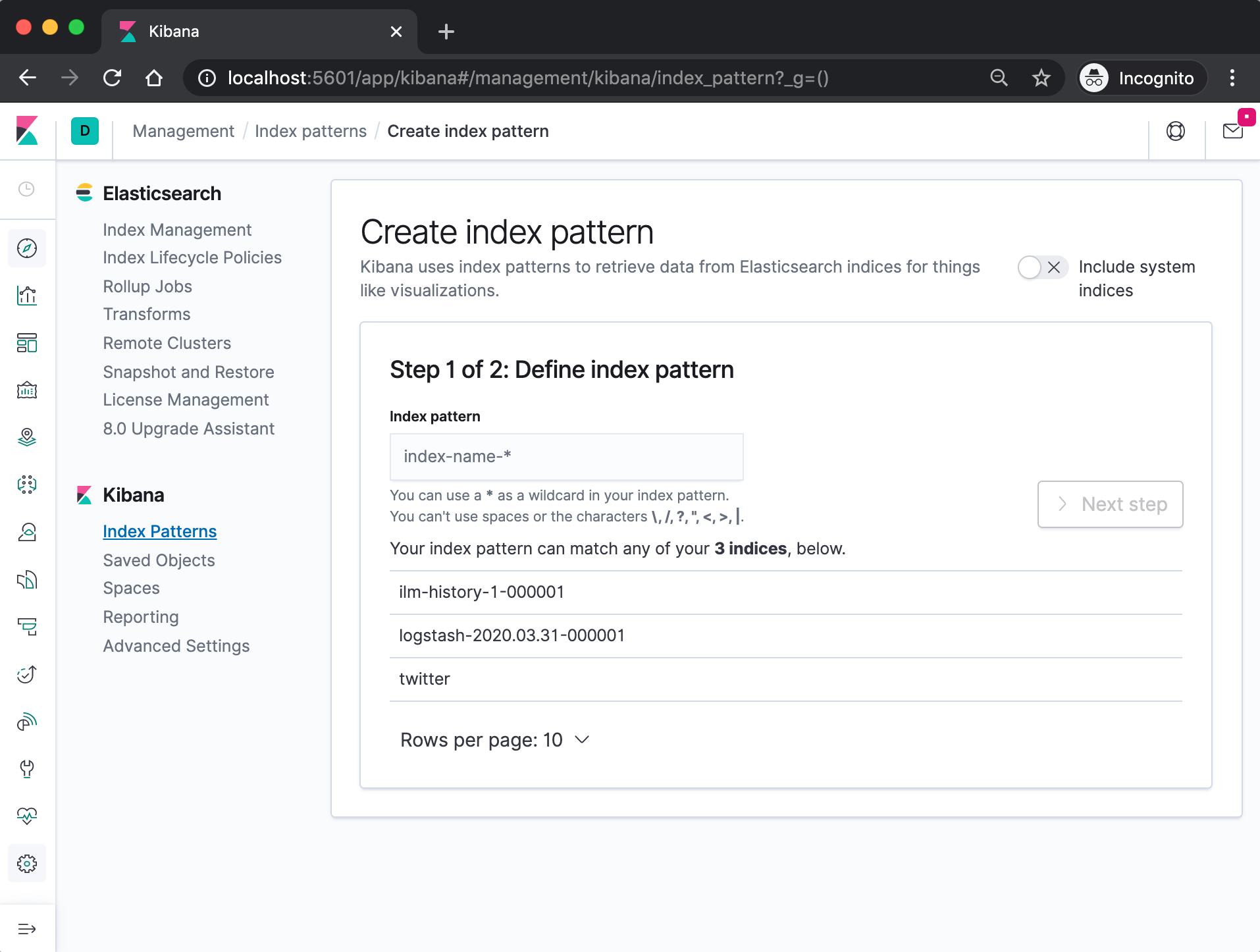
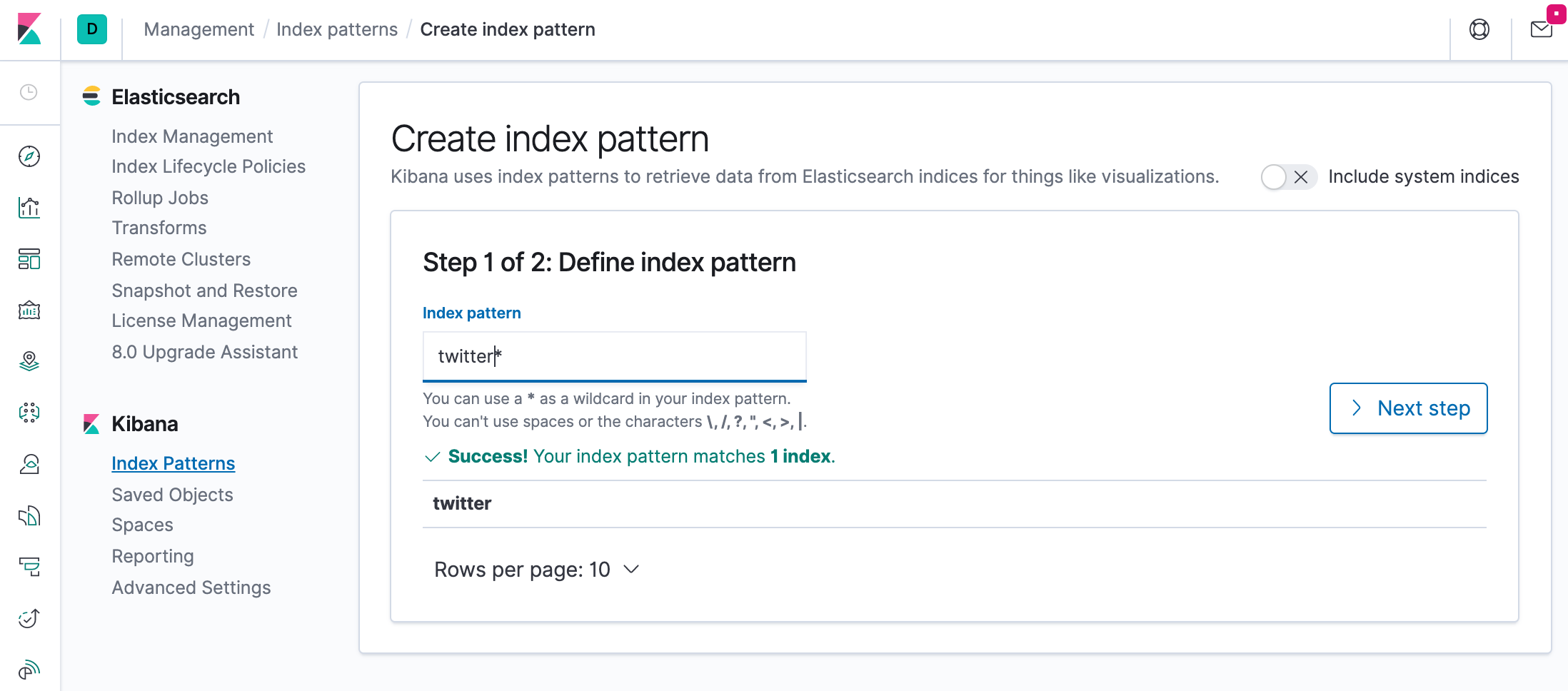
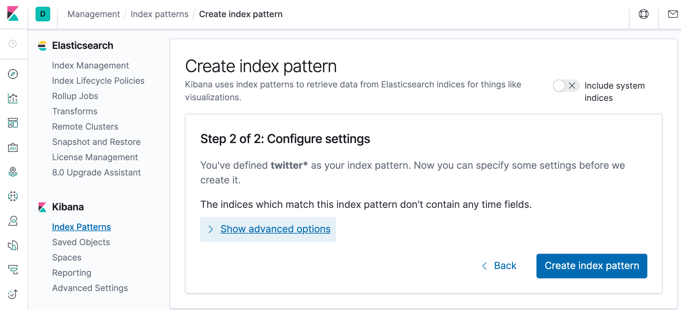
Specify an index pattern that matches the name of one or more of our Elasticsearch indices. The pattern can include an asterisk (*) to matches zero or more characters in an index’s name. When filling out our index pattern, any matched indices will be displayed.
Click “Create index pattern” to add the index pattern. This first pattern is automatically configured as the default. When you have more than one index pattern, we can designate which one to use as the default by clicking on the star icon above the index pattern title from Management > Index Patterns.
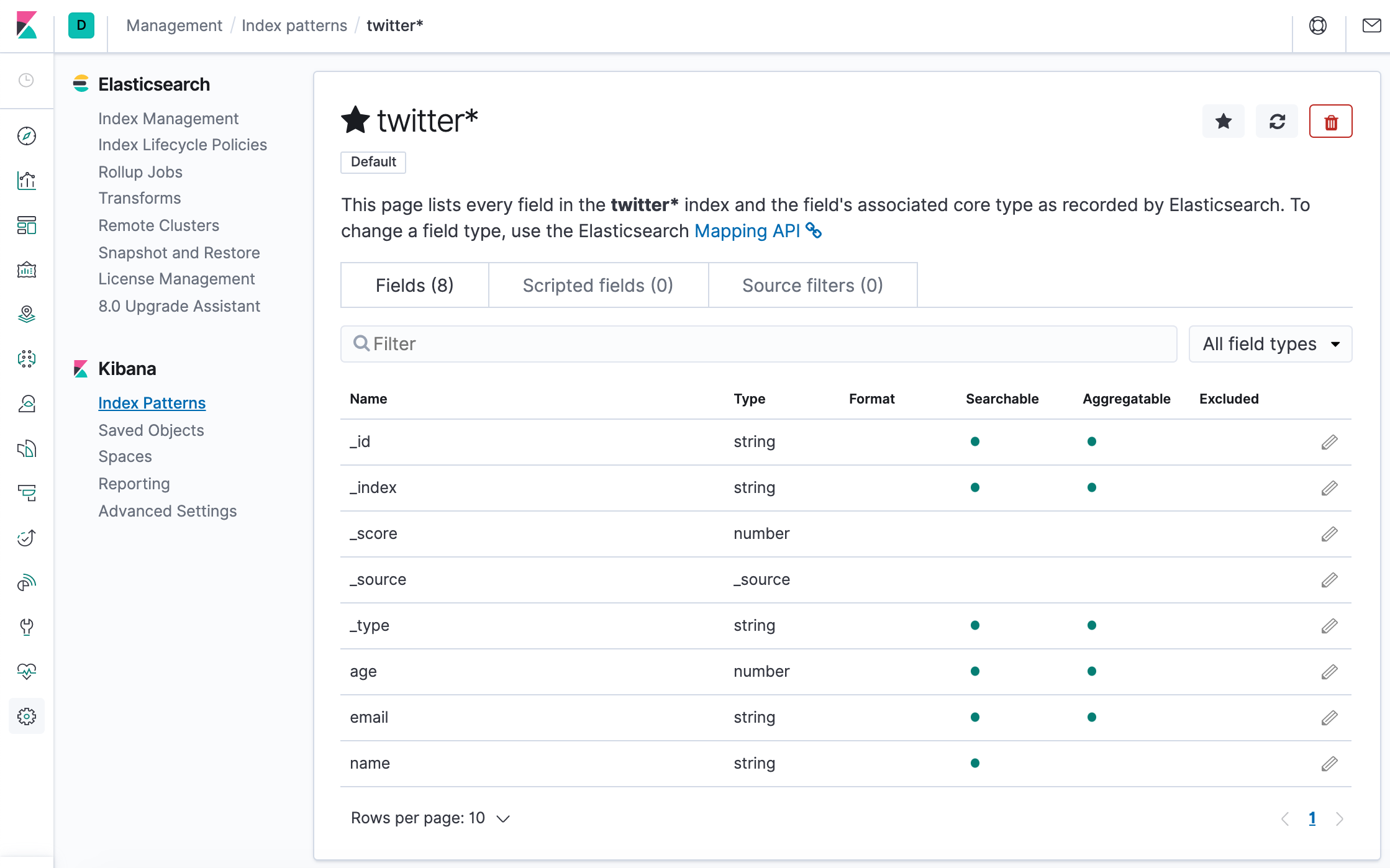
All done! Kibana is now connected to our Elasticsearch data. Kibana displays a read-only list of fields configured for the matching index.
Before we do that, let’s modify the setup for xpack in “elasticsearch/config/elasticsearch.yml” to set “xpack.security.enabled: true”. Otherwise, we may the following error:
{"error":{"root_cause":[{"type":"security_exception","reason":"missing authentication credentials for REST request [/]","header":{"WWW-Authenticate":"Basic realm=\"security\" charset=\"UTF-8\""}}],"type":"security_exception","reason":"missing authentication credentials for REST request [/]","header":{"WWW-Authenticate":"Basic realm=\"security\" charset=\"UTF-8\""}},"status":401}
$ docker-compose up -d
Creating network "einsteinish-elk-stack-with-docker-compose_elk" with driver "bridge"
Creating einsteinish-elk-stack-with-docker-compose_elasticsearch_1 ... done
Creating einsteinish-elk-stack-with-docker-compose_kibana_1        ... done
Creating einsteinish-elk-stack-with-docker-compose_logstash_1      ... done

$ docker-compose ps
                          Name                                         Command               State                                        Ports
-------------------------------------------------------------------------------------------------------------------------------------------------------------------------------------
einsteinish-elk-stack-with-docker-compose_elasticsearch_1   /usr/local/bin/docker-entr ...   Up      0.0.0.0:9200->9200/tcp, 0.0.0.0:9300->9300/tcp
einsteinish-elk-stack-with-docker-compose_kibana_1          /usr/local/bin/dumb-init - ...   Up      0.0.0.0:5601->5601/tcp
einsteinish-elk-stack-with-docker-compose_logstash_1        /usr/local/bin/docker-entr ...   Up      0.0.0.0:5000->5000/tcp, 0.0.0.0:5000->5000/udp, 5044/tcp, 0.0.0.0:9600->9600/tcp
$
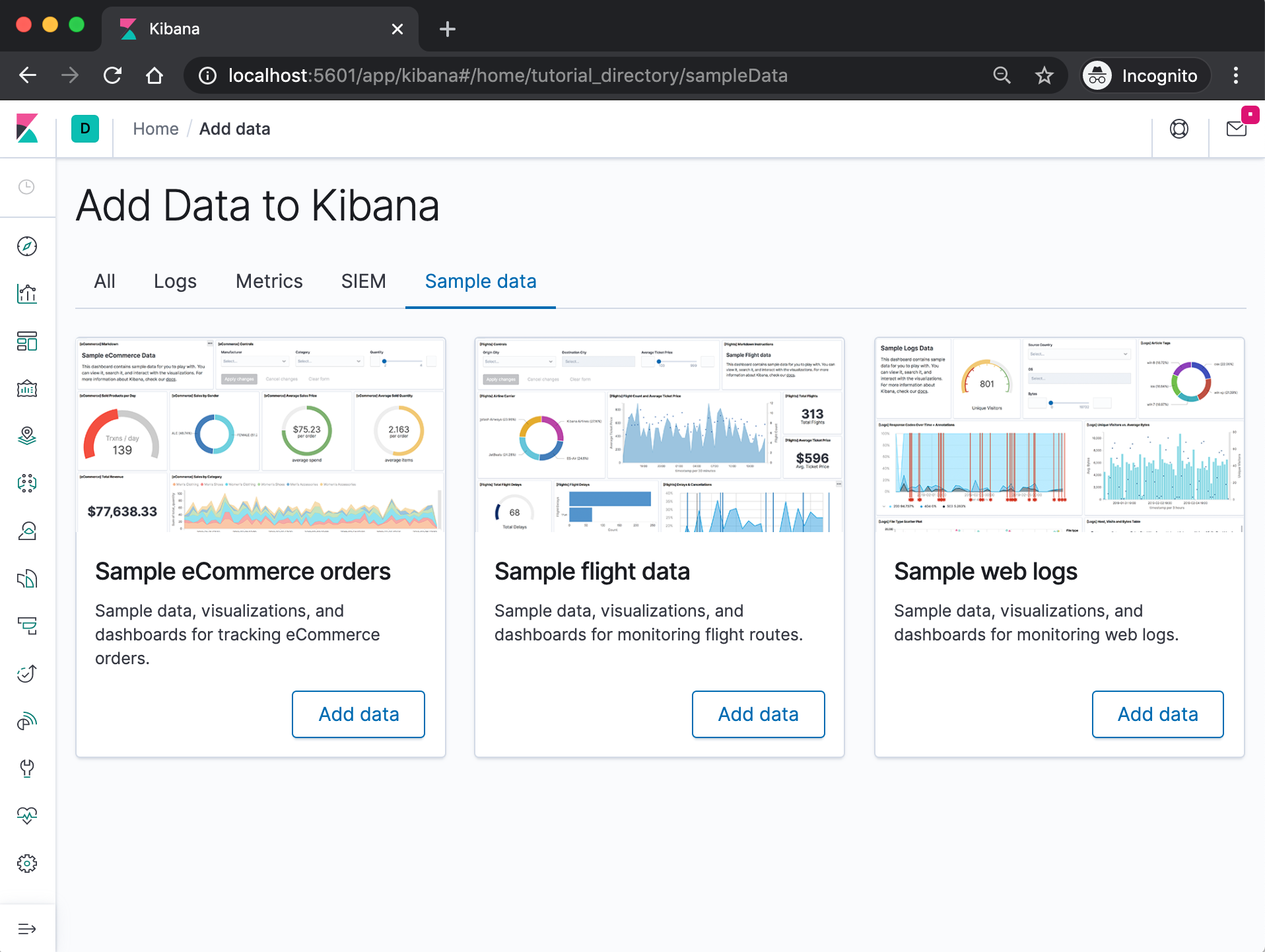
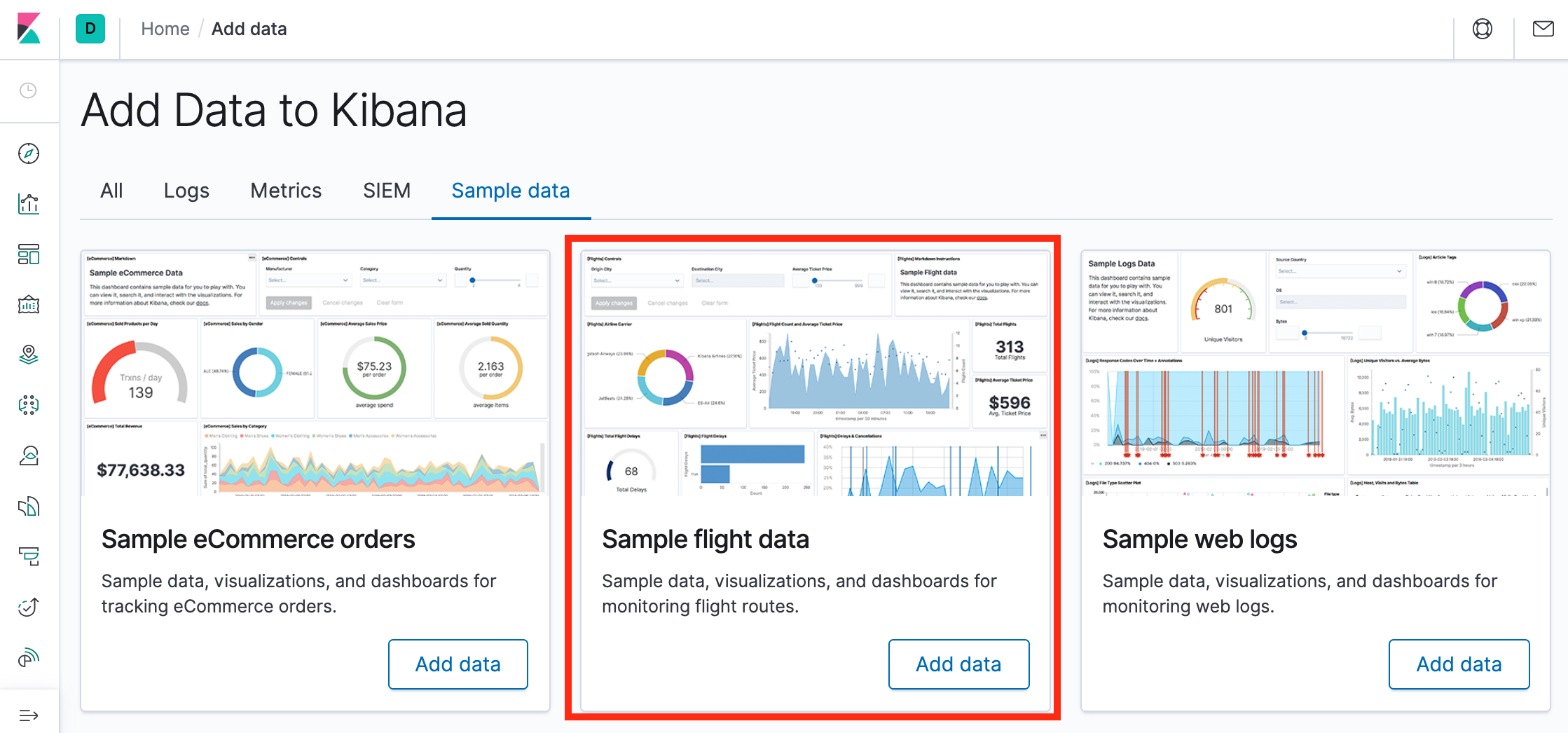
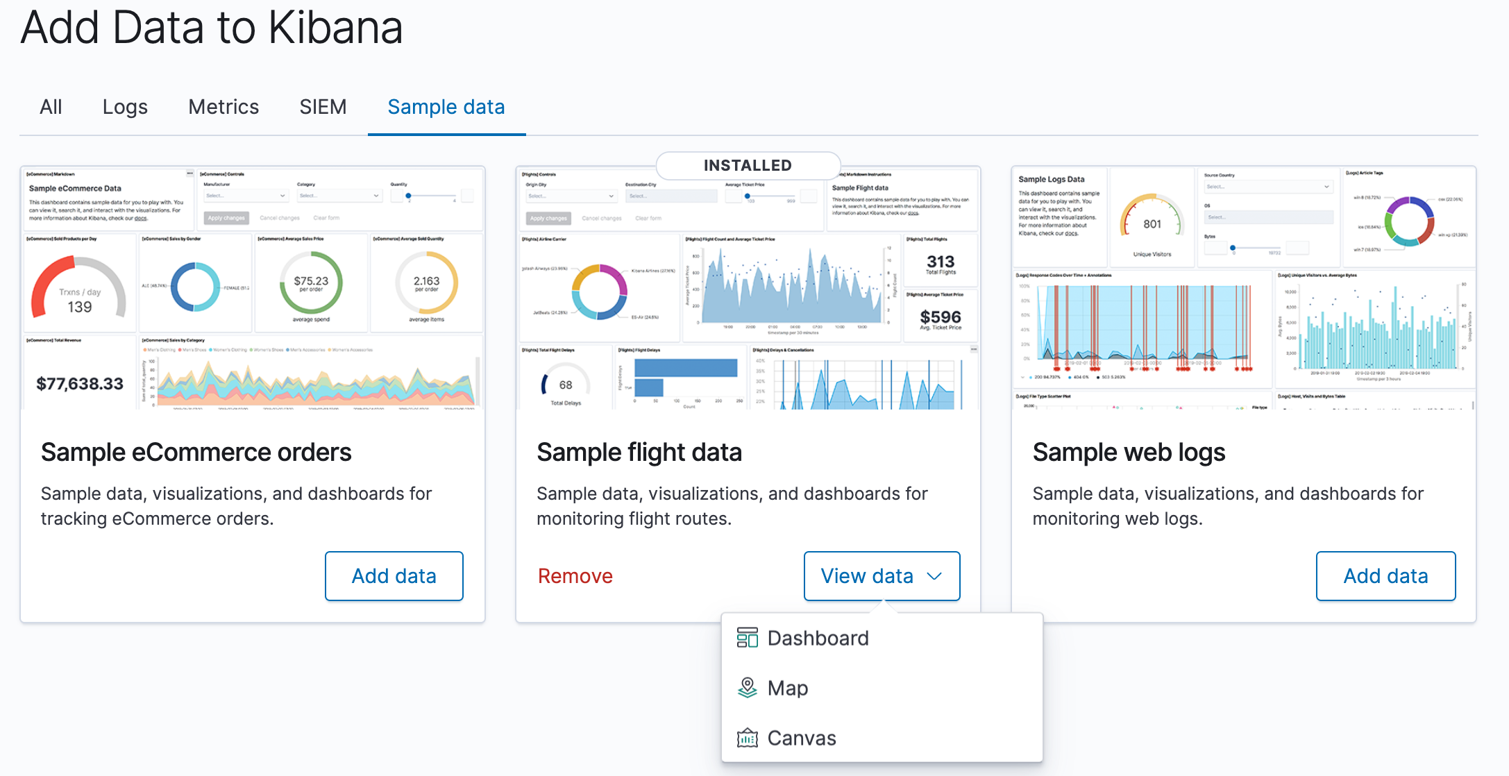
On the Kibana home page, click the link underneath Add sample data.
On the Sample flight data card, click Add data.
Once the data is added, click View data > Dashboard.
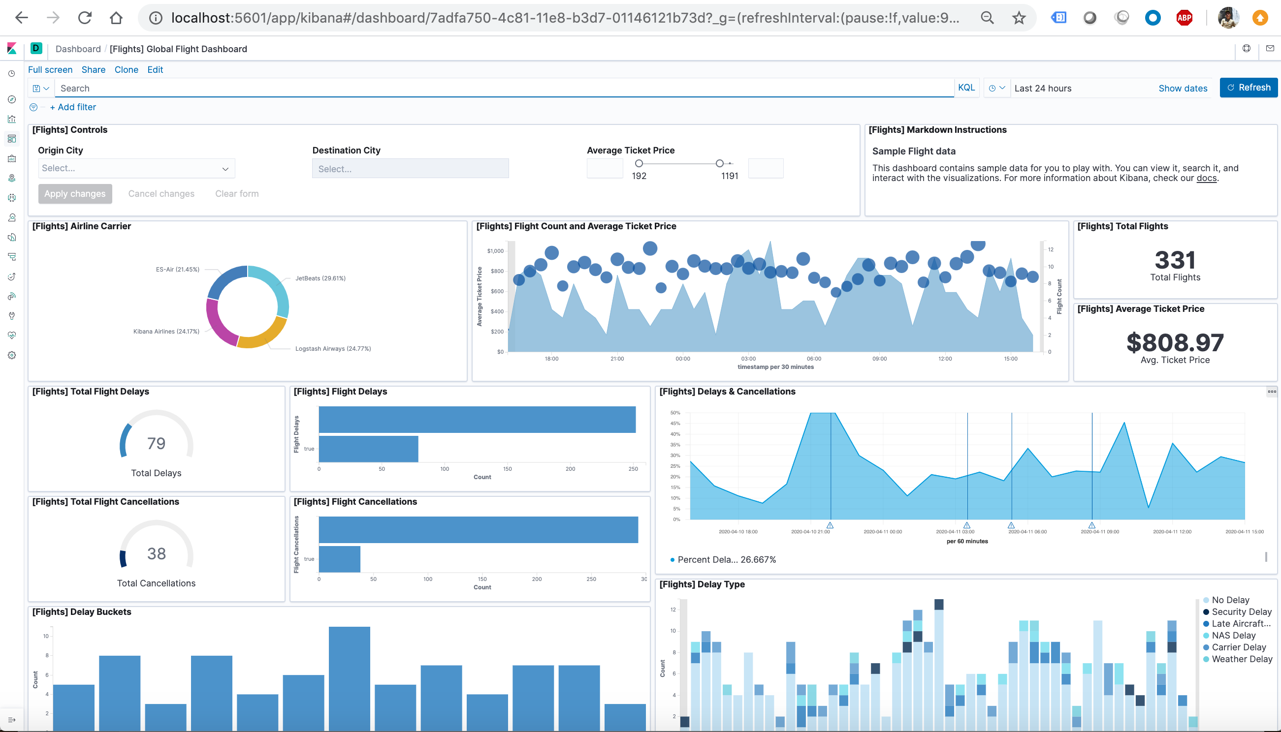
Now, we are on the Global Flight dashboard, a collection of charts, graphs, maps, and other visualizations of the the data in the kibana_sample_data_flights index.
Filtering the Sample Data
In the Controls visualization, set an Origin City and a Destination City.
Click Apply changes. The OriginCityName and the DestCityName fields are filtered to match the data we specified. For example, this dashboard shows the data for flights from London to Oslo.
To add a filter manually, click Add filter in the filter bar, and specify the data we want to view.
When we are finished experimenting, remove all filters.
Querying the Data
To find all flights out of Rome, enter this query in the query bar and click Update:OriginCityName:Rome
For a more complex query with AND and OR, try this: OriginCityName:Rome AND (Carrier:JetBeats OR “Kibana Airlines”)
When finished exploring the dashboard, remove the query by clearing the contents in the query bar and clicking Update.
Discovering the Data
In Discover, we have access to every document in every index that matches the selected index pattern. The index pattern tells Kibana which Elasticsearch index we are currently exploring. We can submit search queries, filter the search results, and view document data.
In the side navigation, click Discover.
Ensure kibana_sample_data_flights is the current index pattern. We might need to click New in the menu bar to refresh the data.
To choose which fields to display, hover the pointer over the list of Available fields, and then click add next to each field we want include as a column in the table. For example, if we add the DestAirportID and DestWeather fields, the display includes columns for those two fields.
Editing Visualization
We have edit permissions for the Global Flight dashboard, so we can change the appearance and behavior of the visualizations. For example, we might want to see which airline has the lowest average fares.
In the side navigation, click Recently viewed and open the Global Flight Dashboard.
In the menu bar, click Edit.
In the Average Ticket Price visualization, click the gear icon in the upper right.
From the Options menu, select Edit visualization.
Create a bucket aggregation
In the Buckets pane, select Add > Split group.
In the Aggregation dropdown, select Terms.
In the Field dropdown, select Carrier.
Set Descending to 4.
Click Apply changes apply changes button.
Save the Visualization
In the menu bar, click Save.
Leave the visualization name as is and confirm the save.
Go to the Global Flight dashboard and scroll the Average Ticket Price visualization to see the four prices.
Optionally, edit the dashboard. Resize the panel for the Average Ticket Price visualization by dragging the handle in the lower right. We can also rearrange the visualizations by clicking the header and dragging. Be sure to save the dashboard.
Inspect the data
Seeing visualizations of our data is great, but sometimes we need to look at the actual data to understand what’s really going on. We can inspect the data behind any visualization and view the Elasticsearch query used to retrieve it.
In the dashboard, hover the pointer over the pie chart, and then click the icon in the upper right.
From the Options menu, select Inspect. The initial view shows the document count.
To look at the query used to fetch the data for the visualization, select View > Requests in the upper right of the Inspect pane.
Remove the sample data set
When we’re done experimenting with the sample data set, we can remove it.
Kafka is an open source software for streaming data, which you can get more infomation about it here: https://kafka.apache.org
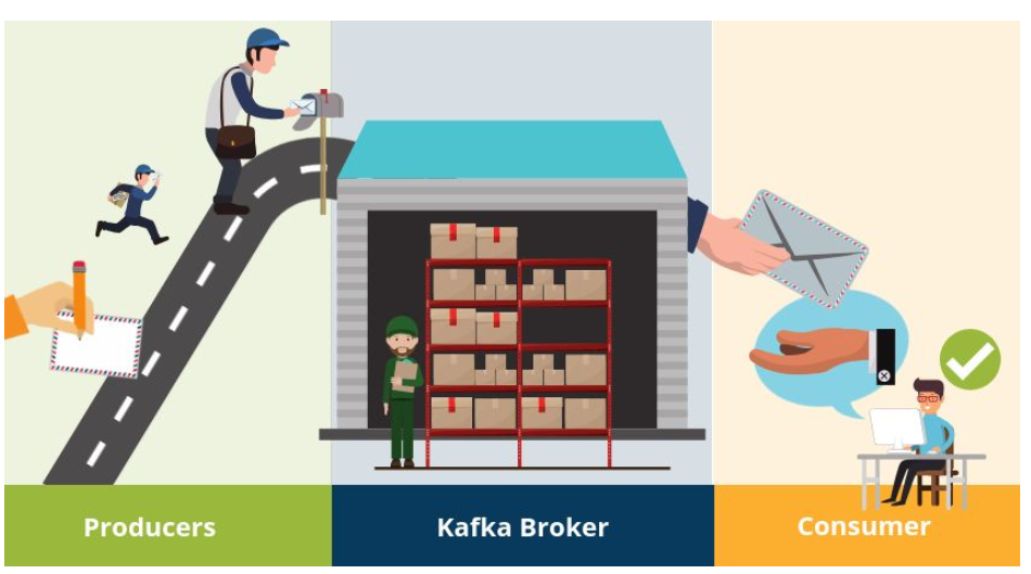
Apache Kafka is a publish-subscribe (pub-sub) message system that allows messages (also called records) to be sent between processes, applications, and servers. Simply said – Kafka stores streams of records. A record can include any kind of information. It could, for example, have information about an event that has happened on a website or could be a simple text message that triggers an event so another application may connect to the system and process or reprocess it. Unlike most messaging systems, the message queue in Kafka (also called a log) is persistent. The data sent is stored until a specified retention period has passed by. Noticeable for Apache Kafka is that records are not deleted when consumed. An Apache Kafka cluster consists of a chosen number of brokers/servers (also called nodes). Apache Kafka itself is storing streams of records. A record is data containing a key, value and timestamp sent from a producer. The producer publishes records on one or more topics. You can think of a topic as a category to where, applications can add, process and reprocess records (data). Consumers can then subscribe to one or more topics and process the stream of records. Kafka is often used when building applications and systems in need of real-time streaming.
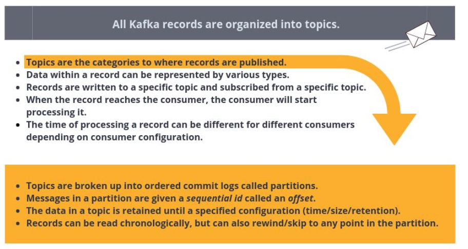
Topics and Data Streams
All Kafka records are organized into topics. Topics are the categories in the Apache Kafka broker to where records are published. Data within a record can be of various types, such as String or JSON. The records are written to a specific topic by a producer and subscribed from a specific topic by a consumer. All Kafka records are organized into topics. Topics are the categories in the Apache Kafka broker where records are published. Data within a record can consist of various types, such as String or JSON. The records are written to a specific topic by a producer and subscribed from a specific topic by a consumer. When the record gets consumed by the consumer, the consumer will start processing it. Consumers can consume records at a different pace, all depending on how they are configured. Topics are configured with a retention policy, either a period of time or a size limit. The record remains in the topic until the retention period/size limit is exceeded. Partition Kafka topics are divided into partitions which contain records in an unchangeable sequence. A partition is also known as a commit log. Partitions allow you to parallelize a topic by splitting the data into a topic across multiple nodes. Each record in a partition is assigned and identified by its unique offset . This offset points to the record in a partition. Incoming records are appended at the end of a partition. The consumer then maintains the offset to keep track of the next record to read. Kafka can maintain durability by replicating the messages to different brokers (nodes). A topic can have multiple partitions. This allows multiple consumers to read from a topic in parallel. The producer decides which topic and partition the message should be placed on.
PRACTICLE INSTALL KAFKA:
Installation
In this article, I am going to explain how to install Kafka on Ubuntu. To install Kafka, Java must be installed on your system. It is a must to set up ZooKeeper for Kafka. ZooKeeper performs many tasks for Kafka but in short, we can say that ZooKeeper manages the Kafka cluster state.
Unzip the file. Inside the conf directory, rename the file zoo_sample.cfgas zoo.cfg.
The zoo.cfg file keeps configuration for ZooKeeper, i.e. on which port the ZooKeeper instance will listen, data directory, etc.
The default listen port is 2181. You can change this port by changing clientPort.
The default data directory is /tmp/data. Change this, as you will not want ZooKeeper’s data to be deleted after some random timeframe. Createa folder with the name datain the ZooKeeper directory and change the dataDirin zoo.cfg.
Go to the bin directory.
Start ZooKeeper by executing the command ./zkServer.sh start.
Stop ZooKeeper by stopping the command ./zkServer.sh stop.
Kafka Setup
Download the latest stable version of Kafka from here.
Unzip this file. The Kafka instance (Broker) configurations are kept in the config directory.
Go to the config directory. Open the file server.properties.
Remove the comment from listeners property, i.e. listeners=PLAINTEXT://:9092. The Kafka broker will listen on port 9092.
Change log.dirs to /kafka_home_directory/kafka-logs.
Check the zookeeper.connect property and change it as per your needs. The Kafka broker will connect to this ZooKeeper instance.
Go to the Kafka home directory and execute the command ./bin/kafka-server-start.sh config/server.properties.
Stop the Kafka broker through the command ./bin/kafka-server-stop.sh.
Kafka Broker Properties
For beginners, the default configurations of the Kafka broker are good enough, but for production-level setup, one must understand each configuration. I am going to explain some of these configurations.
broker.id: The ID of the broker instance in a cluster.
zookeeper.connect: The ZooKeeper address (can list multiple addresses comma-separated for the ZooKeeper cluster). Example: localhost:2181,localhost:2182.
zookeeper.connection.timeout.ms: Time to wait before going down if, for some reason, the broker is not able to connect.
Socket Server Properties
socket.send.buffer.bytes: The send buffer used by the socket server.
socket.receive.buffer.bytes: The socket server receives a buffer for network requests.
socket.request.max.bytes: The maximum request size the server will allow. This prevents the server from running out of memory.
Flush Properties
Each arriving message at the Kafka broker is written into a segment file. The catch here is that this data is not written to the disk directly. It is buffered first. The below two properties define when data will be flushed to disk. Very large flush intervals may lead to latency spikes when the flush happens and a very small flush interval may lead to excessive seeks.
log.flush.interval.messages: Threshold for message count that is once reached all messages are flushed to the disk.
log.flush.interval.ms: Periodic time interval after which all messages will be flushed into the disk.
Log Retention
As discussed above, messages are written into a segment file. The following policies define when these files will be removed.
log.retention.hours: The minimum age of the segment file to be eligible for deletion due to age.
log.retention.bytes: A size-based retention policy for logs. Segments are pruned from the log unless the remaining segments drop below log.retention.bytes.
log.segment.bytes: Size of the segment after which a new segment will be created.
log.retention.check.interval.ms: Periodic time interval after which log segments are checked for deletion as per the retention policy. If both retention policies are set, then segments are deleted when either criterion is met.