High availability with corosync and pacemaker

Once upon a time, I need to setup High Availability for my servers. I have 2 servers: 1 main server, let’s say A (with public IP, for example 1.0.0.1, private IP: 2.0.0.1) and 1 backup server, let’s say B (with public IP 1.0.0.2 , private IP: 2.0.0.2) and I have a public IP (1.0.0.3) which is used as the IP for my programmed APIs. Two servers are in the same private network.

Goal

Server A and B run with an active/passive configuration. Server A always take public IP (1.0.0.3), whenever server A is down, server B will take this public IP and become the main server.

Solution

After some researches, I decided to use Corosync and Pacemaker to setup the High Availability for my servers.

Corosync is an open source program that provides cluster membership and messaging capabilities, often referred to as the messaging layer, to client servers.

Pacemaker is an open source cluster resource manager (CRM), a system that coordinates resources and services that are managed and made highly available by a cluster. In essence, Corosync enables servers to communicate as a cluster, while Pacemaker provides the ability to control how the cluster behaves.

Synchronizing time betweenservers

Whenever you have multiple servers communicating with each other, especially with clustering software, it is important to ensure their clocks are synchronized. Let’s use NTP (Network Time Protocol) to synchronize our servers. On two servers, run those commands, select the same timezone on both servers:

Configure Firewall

Corosync uses UDP transport between ports 5404, 5405 and 5406 . If you are running a firewall, ensure that communication on those ports are allowed between the servers.

If you use ufw, you could allow traffic on these ports with these commands on both servers:

Or if you use iptables, you could allow traffic on these ports and eth1 (the private network interface) with these commands:

Install Corosync and Pacemaker

Corosync is a dependency of Pacemaker, so we can install both of them using one command. Run this command on both servers:

Configure Authorization Key for two servers

Corosync must be configured so that our servers can communicate as a cluster.

On server A (main server), run these commands:

This will generate a 128-byte cluster authorization key, and write it to /etc/corosync/authkey on server A. Now we need to run this command on server A to copy the authkey to server B (backup server)

Then, on server B, run thoses commands:

Configure Corosync cluster

On both servers, open the corosync.conf and write the below scripts:

You can try to read the scripts and try to understand it. If you can’t, just forget about it :). There are only something that’s you need to remember:

  • server_A_private_IP_address: Private IP of server A
  • server_B_private_IP_address: Private IP of server B
  • private_binding_IP_address: The private IP that’s both server A and B are binding to). To know this address, just run ifconfig on server A (or server B) and take a look at the private interface (usually eth1), you will see something like below, the IP 2.0.0.255 is the value for private_binding_IP_address, because 2 server are running in the same private network, this value must be the same on both server:

Enable and run Corosync

Next, we need to configure Corosync to allow the Pacemaker service. On both servers, create the pcmk file in the Corosync’s service directory with below commands:

Then add this scripts to the pcmkfile

Finally, open file /etc/default/corosync and add this line (if there is already a line START=no, change it to YES as below)

Now, start Corosync on both server

Let’s check if everything is working ok with command:

This should output something like this (if not, wait 1 minute and run the command again):

Enable and Start Pacemaker

Pacemaker, which depends on the messaging capabilities of Corosync, is now ready to be started. On both servers, enable Pacemaker to start on system boot with this command:

Because Pacemaker need to start after Corosync, we set Pacemaker’s start priority to 20, which is higher than Corosync‘s (it’s 19 by default).

Now let’s start Pacemaker:

To interact with Pacemaker, we will use the crm utility. Check Pacemaker’s status:

This should output something like this (if not, wait for 30 seconds and run the command again):

Configure Pacemaker and add our Public IP as a Resource

First we need to config some properties. We can run Pacemaker (crm) commands from either server, as it automatically synchronizes all cluster-related changes across all member nodes. Let’s try to run those commands on server A

Now we will add our public IP (1.0.0.3) as a Resource with this command:

NOTE: The config resource-stickiness=”100″ means that’s whenever a server take the resource, our public IP (1.0.0.3), because the other server is down, it will take it forever even when the other server is online again.

Check the Pacemaker’s status again with command ‘sudo crm status’ you can see:

So we are having one resource running and the primary node (server A) is taking it. It means server A is handle our public IP (1.0.0.3). To double check this, try to run command:

You should see:

Testing, simulate the situation when server A going down

Now, we try to simulate the situation when server A is down, server B should take the public IP (1.0.0.3) in this case.

Of course you can shutdown server A, but if you really don’t want to shut it down, you can make the primary node become standby with command:

Let’s open server B and check pacemaker status with command ‘sudo crm status’ you should see:

Check the server B’s ip with:

You should see server B is now taking our public IP:

Now, to make the server A online again:

Because we set the resource-stickiness=”100″ we need to make secondary node standby and online again to make primary node take our public IP again as default setting.

Innsbruck: capital of the alps

Starting as a roman army post, moving on as an aristocratic residence city and arranging the Olympic Winter Gems twice! Innsbruck has come a long way and probably can present itself as the capital of the Alps.

Innsbruck, the capital of Tirol, Austria spreads out in the Inn Valley where the river Inn makes a bend north, before continuing east. In the midst of the most alpine state of Austria, the city’s 130.000 inhabitants enjoy a thriving city and all year outdoor adventures. Innsbruck got it’s name from the first bridge across the river Inn, that was constructed in around 1170. A small tradingpost by the river soon grew and the town got its city status already in 1200.

Historic centre

Although the city is smack in the middle of the Alps, it’s sometimes overseen as a tourist destination. Sure, arriving in Tirol in winter, most people head directly for the ski slopes. Nevertheless, it’s definitely worth a visit. The main attraction all year around is the historical centre, which is well preserved. You could easily spend 2-3 hours taking in the sites here, which are all within short walking distance. No matter the time of the year, strolling around the historical centre is a delight. The narrow lanes can be crowded at time, but if you opt for an early morning stroll, you can enjoy the sights in peace.

City views

Start by getting up in the City Tower (Stadtturm) to get an overview over the city. The tower, constructed in 1450 A.D, gives you nice views of Innsbruck and the surrounding mountains. OK, you have to go up 148 stairs to reach the viewing platform, but it’s worth the effort. Since the tower is right next the old market square, you get a different impression of some of Innsbruck’s landmarks. Such as the famous Golden Roof, where the shiny appearance comes from the copper slates. The balcony with the roof was built to mark the wedding of emperor Maximillian II and Bianca Maria Sforza in 1500 A.D. The couple used the roofed balcony to watch festivals and knights tournaments.

Even though Innsbruck’s main attraction is the medieval centre, there are a few landmarks in the neighbouring streets as well. Just like Paris and Rome, Innsbruck also has a Triumphal Arch (Triumphpforte). Built in 1765 and located in Maria-Theresien-Straße, not to celebrate victory in war, but for the occasion of the wedding of Archduke Leopold to the Spanish princess, Maria Luisa.

Green retreats

The historical centre is very popular among tourists from all around the world, and especially in summer, it can get very crowded. Nonetheless, if you need to get away from the hoards there are several opportunities. Just a few steps away from the most bustling streets of the old city we found a little park to relax, next to the Jesuit Church. Moreover, if you like hanging out in parks, you could also head for Schlosspark Ambras, which has a very nice park. Especially on hot summer days, the big trees offer shady retreats and plenty of space for the kids to play around. The kids will also probably enjoy the Alpenzoo more than some boring old houses. The Zoo houses a range of animals found in Austria and the Alps.

Advertisement

Snow wonderland

In winter, Tirol and Innsbruck is all about skiing and other snow activities. Innsbruck hosted the 1964 and 1976 Winter Olympics and the slopes are reachable by cable car from the city outskirts. There are several ski resorts very near Innsbruck. Nordkette – the mountain range just north of the city can be reached by metro from the centre and then you change to a cable car in the outskirts of Innsbruck. The Nordkette mountain range is part of Austria’s largest nature park, the Karwendel Nature Park. The Nordkettebahn runs all year and you get phenomenal views from the peak near Hafelekar cable car station  at 2,269 metres above sea level.

Hiking heaven

In summer, Innsbruck is an excellent base for hiking in the surrounding mountains. Some of the cable cars are running in the summer as well, giving easy access to the mountain ranges both north and south of the city. Right in the vincinity of the city you have the Patscherkofel Cable Car which takes you up to just short of 2000 metres above sea level, where you find numerous hiking trails. Furthermore, the view from the top is simply mesmorizing. Also worth a visit is the small but interesting alpine botanic garden Alpengarten Patscherkofel not far from the cable car station , which is run by the University of Innsbruck.

Boots off

Innsbruck is more than just a hub for outdoor activities. Get your hiking or ski boots off and head for the city centre. The city is sizeable enough to have a wide range of dining, cultural and shopping activities, catering for most tastes and wallets. The historical city centre of Innsbruck, as so many others in Austria, is a very lively place. Although most mainstream shops have moved out to one of the shopping malls, there are ample of shopping possibilities in the city centre. Thus, for a rainy day or an afternoon, the city will keep you busy with indoor activities as well.

Lidar technology basics

LiDAR stands for Light Detection and Ranging. It measures distance by sending out laser pulses and calculating how long the reflected light takes to return. This makes LiDAR a powerful sensor for building 3D representations of the environment.

How LiDAR Works

The basic principle is simple: emit light, measure return time, and convert that into distance. By repeating this process rapidly across many directions, LiDAR builds a cloud of points that describe the surrounding scene.

A simplified idea looks like this:

distance = speed_of_light * time_of_flight / 2

The division by two is necessary because the pulse travels to the object and back.

Why Engineers Like LiDAR

  • It provides accurate geometric measurements.
  • It works well for mapping and obstacle detection.
  • It can provide dense 3D structure that cameras do not directly measure.

Common Use Cases

  • Autonomous driving: detect vehicles, road edges, and free space.
  • Mobile robotics: SLAM, obstacle avoidance, and localization.
  • Surveying: terrain and structural measurement.
  • Industrial automation: safety zones and dimensional inspection.

2D vs 3D LiDAR

2D LiDAR scans a plane and is common in indoor mobile robots. 3D LiDAR scans many vertical angles and can capture richer scene structure, which is especially useful in outdoor robotics and autonomous vehicles.

Limitations in Practice

  • LiDAR hardware can be expensive.
  • Rain, dust, and reflective surfaces may affect measurements.
  • Point clouds need additional processing before they become actionable information.
  • A strong perception pipeline is still required to interpret raw geometry.

A Practical Example

A self-driving car may use LiDAR to estimate obstacle position and shape around the vehicle. The perception stack clusters the point cloud, tracks nearby objects, and passes those results to prediction and planning modules. In a warehouse robot, a simpler LiDAR may be enough for 2D obstacle detection and map building.

Why Fusion Still Matters

LiDAR is powerful, but no sensor should be treated as perfect. Cameras provide color and semantic detail. Radar works well in adverse weather. IMU and odometry help stabilize motion estimates. Sensor fusion is therefore the practical engineering answer in most real systems.

Final Thoughts

LiDAR is one of the most important sensing technologies in robotics and autonomy because it turns distance measurement into a usable geometric view of the world. Its value is not just in the hardware, but in how well it is integrated into the full system.

Which programming language should you learn

Programming languages and computer coding have made life simpler for us. Whether it’s automobiles, banks, home appliances, or hospitals, every aspect of our lives depends on codes. No wonder, coding is one of the core skills required by most well-paying jobs today. Coding skills are especially of value in the IT, data analytics, research, web designing, and engineering segments. 

So, which programming languages will continue to be in demand in 2020 and beyond? How many languages should you know to pursue your dream career? We will attempt to answer these tricky questions in this post. 

The ever-growing list of programming languages and protocols can make it tough for programmers and developers to pick any one language that’s most suitable for their jobs or project at hand. Ideally, every programmer should have knowledge of a language that’s close to the system (C, Go, or C++), a language that’s object-oriented (Java or Python), a functional programming language (Scala), and a powerful scripting language (Python and JavaScript). 

Whether you are aiming at joining a Fortune 500 firm or desire to pursue a work-from-home career in programming, it’s important to know what’s hot in the industry. Here are a few programming languages we recommend for coders who want to make it big in 2020. 
 
Job hunting? Sign up for alerts about the latest openings in tech from our Jobs Board
 

1.  Python

 
Python continues to be one of the best programming languages every developer should learn this year. The language is easy-to-learn and offers a clean and well-structured code, making it powerful enough to build a decent web application. 

Python can be used for web and desktop applications, GUI-based desktop applications, machine learning, data science, and network servers. The programming language enjoys immense community support and offers several open-source libraries, frameworks, and modules that make application development a cakewalk.

For instance, Python offers Django and Flask, popular libraries for web development and TensorFlow, Keras, and SciPy for data science applications. 

Though Python has been around for a while, it makes sense to learn this language in 2020 as it can help you get a job or a freelance project quickly, thereby accelerating your career growth. 
 

2.  Kotlin


Kotlin is a general-purpose programming language with type inference. It is designed to be completely interoperable with Java. Moreover, from the time Android announced it as its first language, Kotlin offers features that developers ask for. It effortlessly combines object-oriented and functional programming features within it.

kotlin

(Image: Source)

The effortless interoperation between Java and Kotlin makes Android development faster and enjoyable. Since Kotlin addresses the major issues surfaced in Java, several Java apps are rewritten in Kotlin. For instance, brands like Coursera and Pinterest have already moved to Kotlin due to strong tooling support.  

As most businesses move to Kotlin, Google is bound to promote this language more than Java. Hence, Kotlin has a strong future in the Android app development ecosystem.

Kotlin is an easy-to-learn, open-source, and swift language for Android app development that removes any adoption-related barriers. You can use it for Android development, web development, desktop development, and server-side development. Therefore, it’s a must-learn language for programmers and Android app developers in 2020. 
 

3.  Java

 
Java is celebrating its 24th birthday this year and has been one of the most popular programming languages used for developing server-side applications. Java is a practical choice for  developing Android apps as it can be used to create highly functional programs and platforms. 

This object-oriented programming language does not require a specific hardware infrastructure, is easily manageable, and has a good level of security. Moreover, it is easier to learn Java in comparison to languages such as C and C++. No wonder, nearly 90 percent of Fortune 500 firms rely on Java for their desktop applications and backend development projects. 

java

Despite its industry age, the Java is incredibly stable and not heading for retirement anytime soon. This makes Java one of the most desirable languages among programmers in 2020. 
 

4.  JavaScript/ NodeJS

 
JavaScript (also known as NodeJS) is a popular language among developers who need to work on server-side and client-side programming. It is compatible with several other programming languages, allowing you to create animations, set up buttons, and manage multimedia. 

Owing to its high speed and regular annual updates, JavaScript is an ultimate hit in the IT domain. Reputed firms like Netflix, Uber, PayPal, and several startups use JavaScript to create dynamic web pages that are secure and fast. In fact, the 2018 Developer Skills Report by HackerRank shares that JavaScript is the top programming skill required by companies today. 

(Image Credit: Source)

JavaScript is omnipresent in today’s digital environment. Hence, learning this language makes complete sense. 
 

5.  TypeScript

 
TypeScript, a superset of JavaScript is an object-oriented language that was introduced to extend the capabilities of JS. The language makes it easy for developers to write and maintain codes. TypeScript offers a complete description of each component of the code and can be used for developing large applications with a strict syntax and fewer errors. 

Further, it is well-structured and easy to learn. Its extended toolbox makes application development quick. Owing to the benefits it offers, TypeScript is expected to supercede JS in 2020, making it one of the most sought-after programming languages in the future. 
 

6.  Go

 
Go is fairly a new system-level programming language that has a focused vocabulary and simple scoping rules. It blends the best aspects of functional programming and object-oriented styles. Go is the fastest-growing language on Github, meant to replace languages like Java and C++. 

Stack Overflow survey reveals that Go is the fifth most preferred language among developers today. This is because, Go solves issues like slow compilation and execution in large distributed software systems. 

(Image Credit: Source)

This speed advantage has made Go a critical component of cloud infrastructure. So, if you are planning to work in a serverless ecosystem, Go is the language for you. 
 

7.  Swift

 
Swift is a general-purpose compiled programming language developed by Apple that offers developers a simple and cohesive syntax. It is deeply influenced by Python and Ruby that’s fast, secure, and easy-to-learn. Owning to its versatility and practical applications, Swift has replaced Objective-C as the main language for Apple-related applications. 

Further, since Swift is promoted by Apple, its popularity and community support is increasing. In fact, a study of the top 110 apps on the app store showed that 42 percent of apps are already using Swift. 

swift

(Image Credit: Source)

Coders with little or zero experience can use Swift Playgrounds to learn the language, experiment with complex codes, and work on native iOS and macOS apps. Swift is the premiere coding language that helps developers create iOS apps within a short time. The programming language opens several opportunities for new programmers, allowing them to make it big in the world of app development. 

There is a giant market out there for iOS and you definitely want to be a part of it. If you are eyeing this burgeoning market, Swift is the language you should learn in 2020. 
 
Summing Up
 
Nearly all coders have an insatiable thirst for learning new languages. However, knowing which languages are gaining popularity and can ensure a better career growth will help you prioritize learning them first. Use the information shared in this post to make an informed decision in this matter. 

And more than programming language is nowadays programmer should understand about system administrator, Linux command, Docker, monitoring and testing, because these are very important for your carrier.

Authors:
Truong Thanh Nguyen/ Github: thanh118
Software Developer/ DevOps (Autonomous Driving and Machine Learning)Follow 100 follower · 16 following ·

Frankfurt am Main, Germany
master-engineer.com
@T12Thanh

Understanding pointers in c and c++

Pointers

In earlier chapters, variables have been explained as locations in the computer’s memory which can be accessed by their identifier (their name). This way, the program does not need to care about the physical address of the data in memory; it simply uses the identifier whenever it needs to refer to the variable.

For a C++ program, the memory of a computer is like a succession of memory cells, each one byte in size, and each with a unique address. These single-byte memory cells are ordered in a way that allows data representations larger than one byte to occupy memory cells that have consecutive addresses.

This way, each cell can be easily located in the memory by means of its unique address. For example, the memory cell with the address 1776 always follows immediately after the cell with address 1775 and precedes the one with 1777, and is exactly one thousand cells after 776 and exactly one thousand cells before 2776.

When a variable is declared, the memory needed to store its value is assigned a specific location in memory (its memory address). Generally, C++ programs do not actively decide the exact memory addresses where its variables are stored. Fortunately, that task is left to the environment where the program is run – generally, an operating system that decides the particular memory locations on runtime. However, it may be useful for a program to be able to obtain the address of a variable during runtime in order to access data cells that are at a certain position relative to it.

Address-of operator (&)

The address of a variable can be obtained by preceding the name of a variable with an ampersand sign (&), known as address-of operator. For example:

 
foo = &myvar;

This would assign the address of variable myvar to foo; by preceding the name of the variable myvar with the address-of operator (&), we are no longer assigning the content of the variable itself to foo, but its address.

The actual address of a variable in memory cannot be known before runtime, but let’s assume, in order to help clarify some concepts, that myvar is placed during runtime in the memory address 1776.

In this case, consider the following code fragment:

1
2
3
myvar = 25;
foo = &myvar;
bar = myvar;

The values contained in each variable after the execution of this are shown in the following diagram:

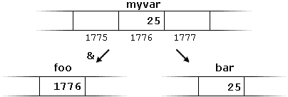
First, we have assigned the value 25 to myvar (a variable whose address in memory we assumed to be 1776).

The second statement assigns foo the address of myvar, which we have assumed to be 1776.

Finally, the third statement, assigns the value contained in myvar to bar. This is a standard assignment operation, as already done many times in earlier chapters.

The main difference between the second and third statements is the appearance of the address-of operator (&).

The variable that stores the address of another variable (like foo in the previous example) is what in C++ is called a pointer. Pointers are a very powerful feature of the language that has many uses in lower level programming. A bit later, we will see how to declare and use pointers.

Dereference operator (*)

As just seen, a variable which stores the address of another variable is called a pointer. Pointers are said to “point to” the variable whose address they store.

An interesting property of pointers is that they can be used to access the variable they point to directly. This is done by preceding the pointer name with the dereference operator (*). The operator itself can be read as “value pointed to by”.

Therefore, following with the values of the previous example, the following statement:

 
baz = *foo;

This could be read as: “baz equal to value pointed to by foo“, and the statement would actually assign the value 25 to baz, since foo is 1776, and the value pointed to by 1776 (following the example above) would be 25.


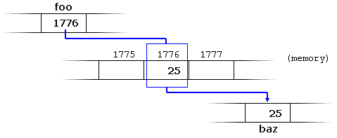
It is important to clearly differentiate that foo refers to the value 1776, while *foo (with an asterisk * preceding the identifier) refers to the value stored at address 1776, which in this case is 25. Notice the difference of including or not including the dereference operator (I have added an explanatory comment of how each of these two expressions could be read):

1
2
baz = foo;   // baz equal to foo (1776)
baz = *foo;  // baz equal to value pointed to by foo (25)  

The reference and dereference operators are thus complementary:

  • & is the address-of operator, and can be read simply as “address of”
  • * is the dereference operator, and can be read as “value pointed to by”

Thus, they have sort of opposite meanings: An address obtained with & can be dereferenced with *.

Earlier, we performed the following two assignment operations:

1
2
myvar = 25;
foo = &myvar;

Right after these two statements, all of the following expressions would give true as result:

1
2
3
4
myvar == 25
&myvar == 1776
foo == 1776
*foo == 25

The first expression is quite clear, considering that the assignment operation performed on myvar was myvar=25. The second one uses the address-of operator (&), which returns the address of myvar, which we assumed it to have a value of 1776. The third one is somewhat obvious, since the second expression was true and the assignment operation performed on foo was foo=&myvar. The fourth expression uses the dereference operator (*) that can be read as “value pointed to by”, and the value pointed to by foo is indeed 25.

So, after all that, you may also infer that for as long as the address pointed to by foo remains unchanged, the following expression will also be true:

 
*foo == myvar

Declaring pointers

Due to the ability of a pointer to directly refer to the value that it points to, a pointer has different properties when it points to a char than when it points to an int or a float. Once dereferenced, the type needs to be known. And for that, the declaration of a pointer needs to include the data type the pointer is going to point to.

The declaration of pointers follows this syntax:

type * name;

where type is the data type pointed to by the pointer. This type is not the type of the pointer itself, but the type of the data the pointer points to. For example:

1
2
3
int * number;
char * character;
double * decimals;

These are three declarations of pointers. Each one is intended to point to a different data type, but, in fact, all of them are pointers and all of them are likely going to occupy the same amount of space in memory (the size in memory of a pointer depends on the platform where the program runs). Nevertheless, the data to which they point to do not occupy the same amount of space nor are of the same type: the first one points to an int, the second one to a char, and the last one to a double. Therefore, although these three example variables are all of them pointers, they actually have different types: int*char*, and double* respectively, depending on the type they point to.

Note that the asterisk (*) used when declaring a pointer only means that it is a pointer (it is part of its type compound specifier), and should not be confused with the dereference operator seen a bit earlier, but which is also written with an asterisk (*). They are simply two different things represented with the same sign.

Let’s see an example on pointers:

1
2
3
4
5
6
7
8
9
10
11
12
13
14
15
16
17
// my first pointer
#include <iostream>
using namespace std;

int main ()
{
  int firstvalue, secondvalue;
  int * mypointer;

  mypointer = &firstvalue;
  *mypointer = 10;
  mypointer = &secondvalue;
  *mypointer = 20;
  cout << "firstvalue is " << firstvalue << '\n';
  cout << "secondvalue is " << secondvalue << '\n';
  return 0;
}
firstvalue is 10
secondvalue is 20

Notice that even though neither firstvalue nor secondvalue are directly set any value in the program, both end up with a value set indirectly through the use of mypointer. This is how it happens:

First, mypointer is assigned the address of firstvalue using the address-of operator (&). Then, the value pointed to by mypointer is assigned a value of 10. Because, at this moment, mypointer is pointing to the memory location of firstvalue, this in fact modifies the value of firstvalue.

In order to demonstrate that a pointer may point to different variables during its lifetime in a program, the example repeats the process with secondvalue and that same pointer, mypointer.

Here is an example a little bit more elaborated:

1
2
3
4
5
6
7
8
9
10
11
12
13
14
15
16
17
18
19
20
// more pointers
#include <iostream>
using namespace std;

int main ()
{
  int firstvalue = 5, secondvalue = 15;
  int * p1, * p2;

  p1 = &firstvalue;  // p1 = address of firstvalue
  p2 = &secondvalue; // p2 = address of secondvalue
  *p1 = 10;          // value pointed to by p1 = 10
  *p2 = *p1;         // value pointed to by p2 = value pointed to by p1
  p1 = p2;           // p1 = p2 (value of pointer is copied)
  *p1 = 20;          // value pointed to by p1 = 20
  
  cout << "firstvalue is " << firstvalue << '\n';
  cout << "secondvalue is " << secondvalue << '\n';
  return 0;
}
firstvalue is 10
secondvalue is 20

Each assignment operation includes a comment on how each line could be read: i.e., replacing ampersands (&) by “address of”, and asterisks (*) by “value pointed to by”.

Notice that there are expressions with pointers p1 and p2, both with and without the dereference operator (*). The meaning of an expression using the dereference operator (*) is very different from one that does not. When this operator precedes the pointer name, the expression refers to the value being pointed, while when a pointer name appears without this operator, it refers to the value of the pointer itself (i.e., the address of what the pointer is pointing to).

Another thing that may call your attention is the line:

 
int * p1, * p2;

This declares the two pointers used in the previous example. But notice that there is an asterisk (*) for each pointer, in order for both to have type int* (pointer to int). This is required due to the precedence rules. Note that if, instead, the code was:

 
int * p1, p2;

p1 would indeed be of type int*, but p2 would be of type int. Spaces do not matter at all for this purpose. But anyway, simply remembering to put one asterisk per pointer is enough for most pointer users interested in declaring multiple pointers per statement. Or even better: use a different statement for each variable.

Pointers and arrays

The concept of arrays is related to that of pointers. In fact, arrays work very much like pointers to their first elements, and, actually, an array can always be implicitly converted to the pointer of the proper type. For example, consider these two declarations:

1
2
int myarray [20];
int * mypointer;

The following assignment operation would be valid:

 
mypointer = myarray;

After that, mypointer and myarray would be equivalent and would have very similar properties. The main difference being that mypointer can be assigned a different address, whereas myarray can never be assigned anything, and will always represent the same block of 20 elements of type int. Therefore, the following assignment would not be valid:

 
myarray = mypointer;

Let’s see an example that mixes arrays and pointers:

1
2
3
4
5
6
7
8
9
10
11
12
13
14
15
16
17
// more pointers
#include <iostream>
using namespace std;

int main ()
{
  int numbers[5];
  int * p;
  p = numbers;  *p = 10;
  p++;  *p = 20;
  p = &numbers[2];  *p = 30;
  p = numbers + 3;  *p = 40;
  p = numbers;  *(p+4) = 50;
  for (int n=0; n<5; n++)
    cout << numbers[n] << ", ";
  return 0;
}
10, 20, 30, 40, 50,

Pointers and arrays support the same set of operations, with the same meaning for both. The main difference being that pointers can be assigned new addresses, while arrays cannot.

In the chapter about arrays, brackets ([]) were explained as specifying the index of an element of the array. Well, in fact these brackets are a dereferencing operator known as offset operator. They dereference the variable they follow just as * does, but they also add the number between brackets to the address being dereferenced. For example:

1
2
a[5] = 0;       // a [offset of 5] = 0
*(a+5) = 0;     // pointed to by (a+5) = 0  

These two expressions are equivalent and valid, not only if a is a pointer, but also if a is an array. Remember that if an array, its name can be used just like a pointer to its first element.

Pointer initialization

Pointers can be initialized to point to specific locations at the very moment they are defined:

1
2
int myvar;
int * myptr = &myvar;

The resulting state of variables after this code is the same as after:

1
2
3
int myvar;
int * myptr;
myptr = &myvar;

When pointers are initialized, what is initialized is the address they point to (i.e., myptr), never the value being pointed (i.e., *myptr). Therefore, the code above shall not be confused with:

1
2
3
int myvar;
int * myptr;
*myptr = &myvar;

Which anyway would not make much sense (and is not valid code).

The asterisk (*) in the pointer declaration (line 2) only indicates that it is a pointer, it is not the dereference operator (as in line 3). Both things just happen to use the same sign: *. As always, spaces are not relevant, and never change the meaning of an expression.

Pointers can be initialized either to the address of a variable (such as in the case above), or to the value of another pointer (or array):

1
2
3
int myvar;
int *foo = &myvar;
int *bar = foo;

Pointer arithmetics

To conduct arithmetical operations on pointers is a little different than to conduct them on regular integer types. To begin with, only addition and subtraction operations are allowed; the others make no sense in the world of pointers. But both addition and subtraction have a slightly different behavior with pointers, according to the size of the data type to which they point.

When fundamental data types were introduced, we saw that types have different sizes. For example: char always has a size of 1 byte, short is generally larger than that, and int and long are even larger; the exact size of these being dependent on the system. For example, let’s imagine that in a given system, char takes 1 byte, short takes 2 bytes, and long takes 4.

Suppose now that we define three pointers in this compiler:

1
2
3
char *mychar;
short *myshort;
long *mylong;

and that we know that they point to the memory locations 10002000, and 3000, respectively.

Therefore, if we write:

1
2
3
++mychar;
++myshort;
++mylong;

mychar, as one would expect, would contain the value 1001. But not so obviously, myshort would contain the value 2002, and mylong would contain 3004, even though they have each been incremented only once. The reason is that, when adding one to a pointer, the pointer is made to point to the following element of the same type, and, therefore, the size in bytes of the type it points to is added to the pointer.


This is applicable both when adding and subtracting any number to a pointer. It would happen exactly the same if we wrote:

1
2
3
mychar = mychar + 1;
myshort = myshort + 1;
mylong = mylong + 1;

Regarding the increment (++) and decrement (--) operators, they both can be used as either prefix or suffix of an expression, with a slight difference in behavior: as a prefix, the increment happens before the expression is evaluated, and as a suffix, the increment happens after the expression is evaluated. This also applies to expressions incrementing and decrementing pointers, which can become part of more complicated expressions that also include dereference operators (*). Remembering operator precedence rules, we can recall that postfix operators, such as increment and decrement, have higher precedence than prefix operators, such as the dereference operator (*). Therefore, the following expression:

 
*p++

is equivalent to *(p++). And what it does is to increase the value of p (so it now points to the next element), but because ++ is used as postfix, the whole expression is evaluated as the value pointed originally by the pointer (the address it pointed to before being incremented).

Essentially, these are the four possible combinations of the dereference operator with both the prefix and suffix versions of the increment operator (the same being applicable also to the decrement operator):

1
2
3
4
*p++   // same as *(p++): increment pointer, and dereference unincremented address
*++p   // same as *(++p): increment pointer, and dereference incremented address
++*p   // same as ++(*p): dereference pointer, and increment the value it points to
(*p)++ // dereference pointer, and post-increment the value it points to 

A typical -but not so simple- statement involving these operators is:

 
*p++ = *q++;

Because ++ has a higher precedence than *, both p and q are incremented, but because both increment operators (++) are used as postfix and not prefix, the value assigned to *p is *q before both p and q are incremented. And then both are incremented. It would be roughly equivalent to:

1
2
3
*p = *q;
++p;
++q;

Like always, parentheses reduce confusion by adding legibility to expressions.

Pointers and const

Pointers can be used to access a variable by its address, and this access may include modifying the value pointed. But it is also possible to declare pointers that can access the pointed value to read it, but not to modify it. For this, it is enough with qualifying the type pointed to by the pointer as const. For example:

1
2
3
4
5
int x;
int y = 10;
const int * p = &y;
x = *p;          // ok: reading p
*p = x;          // error: modifying p, which is const-qualified 

Here p points to a variable, but points to it in a const-qualified manner, meaning that it can read the value pointed, but it cannot modify it. Note also, that the expression &y is of type int*, but this is assigned to a pointer of type const int*. This is allowed: a pointer to non-const can be implicitly converted to a pointer to const. But not the other way around! As a safety feature, pointers to const are not implicitly convertible to pointers to non-const.

One of the use cases of pointers to const elements is as function parameters: a function that takes a pointer to non-const as parameter can modify the value passed as argument, while a function that takes a pointer to const as parameter cannot.

1
2
3
4
5
6
7
8
9
10
11
12
13
14
15
16
17
18
19
20
21
22
23
24
25
26
27
28
29
// pointers as arguments:
#include <iostream>
using namespace std;

void increment_all (int* start, int* stop)
{
  int * current = start;
  while (current != stop) {
    ++(*current);  // increment value pointed
    ++current;     // increment pointer
  }
}

void print_all (const int* start, const int* stop)
{
  const int * current = start;
  while (current != stop) {
    cout << *current << '\n';
    ++current;     // increment pointer
  }
}

int main ()
{
  int numbers[] = {10,20,30};
  increment_all (numbers,numbers+3);
  print_all (numbers,numbers+3);
  return 0;
}
11
21
31

Note that print_all uses pointers that point to constant elements. These pointers point to constant content they cannot modify, but they are not constant themselves: i.e., the pointers can still be incremented or assigned different addresses, although they cannot modify the content they point to.

And this is where a second dimension to constness is added to pointers: Pointers can also be themselves const. And this is specified by appending const to the pointed type (after the asterisk):

1
2
3
4
5
int x;
      int *       p1 = &x;  // non-const pointer to non-const int
const int *       p2 = &x;  // non-const pointer to const int
      int * const p3 = &x;  // const pointer to non-const int
const int * const p4 = &x;  // const pointer to const int 

The syntax with const and pointers is definitely tricky, and recognizing the cases that best suit each use tends to require some experience. In any case, it is important to get constness with pointers (and references) right sooner rather than later, but you should not worry too much about grasping everything if this is the first time you are exposed to the mix of const and pointers. More use cases will show up in coming chapters.

To add a little bit more confusion to the syntax of const with pointers, the const qualifier can either precede or follow the pointed type, with the exact same meaning:

1
2
const int * p2a = &x;  //      non-const pointer to const int
int const * p2b = &x;  // also non-const pointer to const int 

As with the spaces surrounding the asterisk, the order of const in this case is simply a matter of style. This chapter uses a prefix const, as for historical reasons this seems to be more extended, but both are exactly equivalent. The merits of each style are still intensely debated on the internet.

Pointers and string literals

As pointed earlier, string literals are arrays containing null-terminated character sequences. In earlier sections, string literals have been used to be directly inserted into cout, to initialize strings and to initialize arrays of characters.

But they can also be accessed directly. String literals are arrays of the proper array type to contain all its characters plus the terminating null-character, with each of the elements being of type const char (as literals, they can never be modified). For example:

 
const char * foo = "hello"; 

This declares an array with the literal representation for "hello", and then a pointer to its first element is assigned to foo. If we imagine that "hello" is stored at the memory locations that start at address 1702, we can represent the previous declaration as:


Note that here foo is a pointer and contains the value 1702, and not 'h', nor "hello", although 1702 indeed is the address of both of these.

The pointer foo points to a sequence of characters. And because pointers and arrays behave essentially in the same way in expressions, foo can be used to access the characters in the same way arrays of null-terminated character sequences are. For example:

1
2
*(foo+4)
foo[4]

Both expressions have a value of 'o' (the fifth element of the array).

Pointers to pointers

C++ allows the use of pointers that point to pointers, that these, in its turn, point to data (or even to other pointers). The syntax simply requires an asterisk (*) for each level of indirection in the declaration of the pointer:

1
2
3
4
5
6
char a;
char * b;
char ** c;
a = 'z';
b = &a;
c = &b;

This, assuming the randomly chosen memory locations for each variable of 72308092, and 10502, could be represented as:


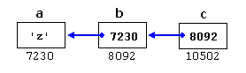
With the value of each variable represented inside its corresponding cell, and their respective addresses in memory represented by the value under them.

The new thing in this example is variable c, which is a pointer to a pointer, and can be used in three different levels of indirection, each one of them would correspond to a different value:

  • c is of type char** and a value of 8092
  • *c is of type char* and a value of 7230
  • **c is of type char and a value of 'z'

void pointers

The void type of pointer is a special type of pointer. In C++, void represents the absence of type. Therefore, void pointers are pointers that point to a value that has no type (and thus also an undetermined length and undetermined dereferencing properties).

This gives void pointers a great flexibility, by being able to point to any data type, from an integer value or a float to a string of characters. In exchange, they have a great limitation: the data pointed to by them cannot be directly dereferenced (which is logical, since we have no type to dereference to), and for that reason, any address in a void pointer needs to be transformed into some other pointer type that points to a concrete data type before being dereferenced.

One of its possible uses may be to pass generic parameters to a function. For example:

1
2
3
4
5
6
7
8
9
10
11
12
13
14
15
16
17
18
19
20
21
// increaser
#include <iostream>
using namespace std;

void increase (void* data, int psize)
{
  if ( psize == sizeof(char) )
  { char* pchar; pchar=(char*)data; ++(*pchar); }
  else if (psize == sizeof(int) )
  { int* pint; pint=(int*)data; ++(*pint); }
}

int main ()
{
  char a = 'x';
  int b = 1602;
  increase (&a,sizeof(a));
  increase (&b,sizeof(b));
  cout << a << ", " << b << '\n';
  return 0;
}
y, 1603

sizeof is an operator integrated in the C++ language that returns the size in bytes of its argument. For non-dynamic data types, this value is a constant. Therefore, for example, sizeof(char) is 1, because char has always a size of one byte.

Invalid pointers and null pointers

In principle, pointers are meant to point to valid addresses, such as the address of a variable or the address of an element in an array. But pointers can actually point to any address, including addresses that do not refer to any valid element. Typical examples of this are uninitialized pointers and pointers to nonexistent elements of an array:

1
2
3
4
int * p;               // uninitialized pointer (local variable)

int myarray[10];
int * q = myarray+20;  // element out of bounds 

Neither p nor q point to addresses known to contain a value, but none of the above statements causes an error. In C++, pointers are allowed to take any address value, no matter whether there actually is something at that address or not. What can cause an error is to dereference such a pointer (i.e., actually accessing the value they point to). Accessing such a pointer causes undefined behavior, ranging from an error during runtime to accessing some random value.

But, sometimes, a pointer really needs to explicitly point to nowhere, and not just an invalid address. For such cases, there exists a special value that any pointer type can take: the null pointer value. This value can be expressed in C++ in two ways: either with an integer value of zero, or with the nullptr keyword:

1
2
int * p = 0;
int * q = nullptr;

Here, both p and q are null pointers, meaning that they explicitly point to nowhere, and they both actually compare equal: all null pointers compare equal to other null pointers. It is also quite usual to see the defined constant NULL be used in older code to refer to the null pointer value:

 
int * r = NULL;

NULL is defined in several headers of the standard library, and is defined as an alias of some null pointer constant value (such as 0 or nullptr).

Do not confuse null pointers with void pointers! A null pointer is a value that any pointer can take to represent that it is pointing to “nowhere”, while a void pointer is a type of pointer that can point to somewhere without a specific type. One refers to the value stored in the pointer, and the other to the type of data it points to.

Pointers to functions

C++ allows operations with pointers to functions. The typical use of this is for passing a function as an argument to another function. Pointers to functions are declared with the same syntax as a regular function declaration, except that the name of the function is enclosed between parentheses () and an asterisk (*) is inserted before the name:

1
2
3
4
5
6
7
8
9
10
11
12
13
14
15
16
17
18
19
20
21
22
23
24
25
26
27
// pointer to functions
#include <iostream>
using namespace std;

int addition (int a, int b)
{ return (a+b); }

int subtraction (int a, int b)
{ return (a-b); }

int operation (int x, int y, int (*functocall)(int,int))
{
  int g;
  g = (*functocall)(x,y);
  return (g);
}

int main ()
{
  int m,n;
  int (*minus)(int,int) = subtraction;

  m = operation (7, 5, addition);
  n = operation (20, m, minus);
  cout <<n;
  return 0;
}
8

In the example above, minus is a pointer to a function that has two parameters of type int. It is directly initialized to point to the function subtraction:

 
int (* minus)(int,int) = subtraction;

Yolo for real-time detection

YOLO, short for You Only Look Once, changed how many engineers think about object detection. Earlier detection systems often used multi-stage pipelines that proposed regions first and classified them later. YOLO reframed detection as a direct prediction problem: take an image, run one forward pass, and predict bounding boxes plus class scores quickly enough for real-time use.

That design choice made YOLO especially attractive in robotics, video analytics, and autonomous systems, where latency matters as much as raw accuracy.

Bounding boxes for object detection example
Object detection is not just classification. The model must also localize the object with a useful bounding box. Source: Wikimedia Commons, Intersection over Union – object detection bounding boxes.jpg.

What problem YOLO solves

Image classification answers a simple question: what is in this image? Detection answers a harder one: what objects are present, where are they, and which class belongs to each box?

That difference matters in real systems. A vehicle or robot does not only need to know that a scene contains a pedestrian. It needs to know where the pedestrian is, how that person moves across frames, and whether the detection is stable enough to influence planning.

YOLO became popular because it made this detection step fast and practical at scale.

Why YOLO became influential

There are three main reasons YOLO spread so widely:

  • Speed: real-time inference made it attractive for video and edge deployment.
  • Simplicity: a single unified detector was easier to explain and deploy than older multi-stage systems.
  • Strong engineering ecosystem: later implementations and tooling made training, exporting, and deployment more accessible.

Over time, the YOLO family evolved a lot. Anchor strategies changed, backbones improved, post-processing changed, and modern variants added tasks such as segmentation, pose, tracking, and oriented boxes. But the core identity remained: detection should be fast enough to use in real systems.

How YOLO works at a practical level

Conceptually, YOLO takes an image and predicts object locations and categories in one inference path. A modern pipeline usually includes:

  1. image resize and normalization
  2. feature extraction with a backbone network
  3. multi-scale detection heads
  4. confidence scoring and class prediction
  5. post-processing to remove duplicate boxes

The exact architecture depends on the version you use, but the operational idea is stable: produce detections quickly enough for downstream systems to react.

from ultralytics import YOLO

model = YOLO("yolo11n.pt")
results = model("street_scene.jpg")

for result in results:
    for box in result.boxes:
        print(box.cls, box.conf, box.xyxy)

The code above looks simple, but the real engineering work is often around dataset quality, deployment constraints, label consistency, camera setup, and tracking across frames.

Where YOLO fits in a larger system

YOLO is rarely the whole perception stack. In a deployed system it usually feeds into something larger:

  • multi-object tracking
  • sensor fusion
  • risk estimation
  • behavior planning
  • alerting or actuation logic

For example, in an autonomous-driving context, YOLO-style detection may identify vehicles, pedestrians, bikes, and traffic cones. But planning still needs temporal tracking, motion prediction, and safety rules before it can turn those detections into driving decisions.

What YOLO is especially good at

YOLO tends to work well when you need:

  • fast detection on live video
  • compact deployment on edge hardware
  • simple integration into monitoring or robotics pipelines
  • good tradeoffs between speed and accuracy

This is why it appears so often in drones, traffic monitoring, warehouse robots, industrial safety, and smart-camera systems.

Where YOLO is not enough by itself

Even a strong detector has limits. YOLO alone does not solve:

  • precise depth estimation
  • fine-grained pixel segmentation
  • long-term tracking identity under heavy occlusion
  • full scene understanding for planning
  • robust performance under severe domain shift without retraining

That is why practical systems usually pair detection with tracking, segmentation, map context, or other sensors.

Real engineering concerns

If you plan to deploy YOLO in a real product, the hard questions are usually not about the marketing benchmark. They are about:

  • label quality and class definitions
  • how often false positives appear in safety-critical scenes
  • how small distant objects can be while still being detected
  • latency on the exact target hardware
  • nighttime, rain, motion blur, or camera vibration
  • monitoring drift after deployment

In many teams, the biggest performance gains come from better data and better deployment choices, not from chasing a new model name every week.

Conclusion

YOLO became influential because it made object detection fast, practical, and easy to integrate into real systems. It remains a strong choice when engineers need real-time perception on images or video. But the best way to use YOLO is to treat it as one reliable module inside a broader perception stack, not as the full system by itself.

References

How self-driving cars work

A self-driving car is not one algorithm and not one sensor. It is a layered system that combines perception, localization, prediction, planning, and control so the vehicle can understand traffic scenes and act safely in real time.

1. Perception

Perception is responsible for answering the question: What is around the car? A self-driving stack may use cameras, LiDAR, radar, ultrasonic sensors, and GPS/IMU inputs. Perception algorithms detect lanes, vehicles, pedestrians, cyclists, traffic signs, and traffic lights.

Modern systems often combine deep learning with geometric tracking. For example, a camera may detect a pedestrian while LiDAR refines shape and distance. Sensor fusion improves reliability because no single sensor is perfect in all conditions.

2. Localization

Localization answers: Where is the car? GPS alone is usually not accurate enough for lane-level autonomy, so self-driving cars often combine GNSS, IMU, wheel odometry, HD maps, and LiDAR or camera-based matching. The goal is to maintain a precise estimate of position and orientation.

3. Prediction

Other road users move unpredictably. Prediction estimates what they may do next. A vehicle ahead may brake. A pedestrian may step onto the road. A cyclist may merge into the lane. The system therefore predicts future trajectories and uncertainties, not only current positions.

4. Behavior Planning

Behavior planning decides the high-level action: keep lane, stop, yield, overtake, or change lanes. It converts traffic understanding into a driving decision that respects safety and road rules.

5. Motion Planning

Once the system knows what behavior it wants, it needs a feasible trajectory. Motion planning generates a path that is safe, smooth, and physically possible for the vehicle. It considers curvature, speed, nearby obstacles, and passenger comfort.

6. Control

The control layer converts the planned trajectory into steering, throttle, and brake commands. Controllers such as PID, MPC, or LQR help the car track the planned path while remaining stable and responsive.

A Driving Example

Imagine the car approaches a slower vehicle in the same lane:

  1. Perception detects the vehicle ahead and estimates distance.
  2. Localization places the ego car accurately on the map.
  3. Prediction estimates whether the other vehicle will continue straight or slow further.
  4. Behavior planning decides whether to follow or change lane.
  5. Motion planning creates a smooth and safe trajectory.
  6. Control executes the maneuver.

Why Building a Self-Driving Car Is Difficult

  • Real traffic is uncertain and full of corner cases.
  • Sensors are noisy and can fail.
  • Decisions must be made in real time.
  • Safety validation is extremely demanding.

Final Thoughts

The best way to understand self-driving technology is to see it as a systems engineering problem. Each module matters, but what matters most is how well the modules work together under real-world conditions.

Poetry and quiet reflection

Poetry has a different purpose from technical writing. It does not try to explain everything directly. Instead, it creates space for feeling, memory, and reflection. That is one reason poetry remains meaningful even in a world dominated by fast information.

Why Poetry Matters

A poem can hold an emotional truth in very few words. It may express longing, beauty, regret, gratitude, or silence more effectively than long description. That compression is part of its power.

Poetry and Inner Life

In daily life, especially for people working in demanding technical or practical environments, poetry offers another rhythm. It slows the mind down. It reminds us that not everything valuable needs to be optimized or measured.

A Personal Thought

I think poetry matters because it keeps a part of life open that should not become mechanical. Even a short verse can create a pause in the middle of a busy world, and sometimes that pause is exactly what we need.

Final Thoughts

Poetry may be brief, but it is rarely small. A few careful lines can stay with a person for years. That is why poetic language continues to matter, even for people whose daily work is built around logic and systems.

Reflections on the condor trilogy

The Condor Trilogy remains one of the most memorable martial arts novel series for many readers because it offers much more than combat and adventure. It combines loyalty, ambition, love, tragedy, history, and personal growth in a way that makes the story feel emotionally larger than its genre label suggests.

Why the Series Endures

What makes the trilogy powerful is not only the world-building, but also the moral complexity of its characters. Heroes are not always pure, and great talent does not always lead to peace. Characters grow through conflict, loss, and responsibility, which gives the story weight beyond entertainment.

Character and Emotion

Many readers remember the series because of its human relationships. Friendship, devotion, sacrifice, and heartbreak are woven into the martial arts setting in a way that feels deeply personal. The emotional layer is one reason the story continues to resonate across generations.

More Than a Martial Arts Story

The trilogy also reflects themes of identity, belonging, national memory, and the tension between personal desire and larger duty. That broader emotional and historical scope is part of what gives the work its lasting influence.

A Personal View

For me, the trilogy stands out because it creates a strong inner atmosphere. Some works stay in memory because of plot twists. Others stay because of the emotional world they build. This series belongs to the second kind.

Final Thoughts

The Condor Trilogy is memorable not only because it is famous, but because it connects action with feeling and legend with humanity. That combination is what gives it real literary life.

Vision-based navigation in practice

Vision-based navigation uses cameras to estimate motion, understand the environment, and help a robot or vehicle move safely through space. It is attractive because cameras are relatively cheap, lightweight, and rich in detail. A single frame can contain landmarks, lane markings, free space, signs, texture, and semantic cues that other sensors may not capture as naturally.

But camera-based navigation is not simply “look at an image and drive.” A practical navigation stack needs stable calibration, time synchronization, robust pose estimation, and a way to recover when the scene becomes ambiguous.

Camera module near windshield for assisted driving
Cameras mounted near the windshield often support lane keeping, road understanding, and navigation cues. Source: Wikimedia Commons, Lane assist.jpg.

What vision-based navigation really does

At a practical level, vision-based navigation answers three questions:

  • Where am I?
  • How am I moving?
  • What is around me, and where can I go next?

Depending on the platform, the answer may rely on visual odometry, landmark tracking, semantic road understanding, stereo depth, or full SLAM. In an indoor robot, the system may rely on features and loop closure. In a road vehicle, it may use cameras for lane geometry, localization cues, and scene semantics while radar, GNSS, IMU, and maps handle complementary tasks.

The core pipeline

A practical camera-navigation pipeline often looks like this:

  1. Capture synchronized images from one or more calibrated cameras.
  2. Extract visual information such as features, edges, segments, landmarks, or semantic masks.
  3. Estimate motion using frame-to-frame correspondences, optical flow, stereo disparity, or learned motion models.
  4. Build or update a map of landmarks, occupancy, or semantic structure.
  5. Fuse with other sensors such as IMU, wheel odometry, GNSS, LiDAR, or radar.
  6. Provide pose and environment estimates to planning and control.

That pipeline may sound straightforward, but every stage can fail if the image stream is noisy, blurred, poorly synchronized, or visually repetitive.

Visual odometry and SLAM

Two ideas appear in almost every camera-navigation system: visual odometry and SLAM.

Visual odometry estimates the motion of the camera by tracking how the scene changes across frames. It is local and continuous. It tells the system how it moved over the last short period of time.

SLAM, or simultaneous localization and mapping, goes further. It tries to build a consistent map while also using that map to improve localization. Loop closure is especially important here. If the robot revisits a known place, the system can reduce drift and relocalize more accurately.

Systems such as ORB-SLAM became influential because they showed that a camera-only pipeline could estimate trajectory in real time across a wide range of environments. Newer systems expanded this idea to stereo, RGB-D, and visual-inertial settings.

navigation stack
    -> synchronized camera frames
    -> feature tracking or semantic perception
    -> relative pose estimate
    -> map update / loop closure
    -> fused state estimate
    -> planner and controller

What cameras are good at in navigation

Cameras are especially useful when the platform needs semantic context in addition to geometry.

  • Road structure: lanes, curbs, drivable area, intersections, merges, and signs.
  • Landmarks: textured features, repeated landmarks, or learned place descriptors.
  • Obstacle understanding: identifying whether something is a car, pedestrian, bike, or static structure.
  • Localization support: map matching and relocalization from known visual features.

This semantic richness is why cameras remain central in ADAS, delivery robots, warehouse systems, and many research platforms.

Monocular, stereo, and multi-camera navigation

Not all vision-based navigation systems see the world the same way.

  • Monocular: lowest cost and simplest hardware, but scale is ambiguous without motion priors or fusion.
  • Stereo: adds depth through disparity, making pose and obstacle reasoning more stable.
  • Multi-camera surround view: improves coverage at intersections, blind spots, and tight maneuvers.
Stereo vision depth concept
Stereo vision converts left-right image disparity into depth cues that improve navigation and obstacle reasoning. Source: Wikimedia Commons, Stereovision.gif.

Monocular systems can still work very well, especially with IMU fusion, but stereo or multi-camera setups reduce ambiguity when metric depth matters.

Why fusion matters

Camera navigation alone can be impressive, but robust deployed systems almost always fuse vision with other sources of information. An IMU helps stabilize short-term motion estimation. Wheel odometry provides a useful prior for ground robots. GNSS helps with large-scale outdoor localization. LiDAR or radar can add stronger geometric constraints under difficult lighting conditions.

The engineering goal is not to replace every other sensor with cameras. The goal is to let cameras contribute what they do best and rely on fusion when ambiguity grows.

Common failure modes

Vision-based navigation fails for understandable reasons, and those failure modes should shape the system design:

  • low light or night scenes reduce usable detail
  • glare, rain, fog, and dirty lenses degrade image quality
  • textureless walls or roads reduce feature quality
  • dynamic crowds or heavy traffic can confuse motion estimation
  • repetitive patterns create false matches
  • timing and calibration errors break the geometry

If a system does not monitor these conditions, it may produce confident but wrong poses. That is one of the main reasons why state estimation and uncertainty reporting matter so much.

A practical engineering checklist

When evaluating a vision-navigation stack, I would check these points first:

  • How well is camera calibration maintained over time?
  • What is the end-to-end latency from sensor capture to pose output?
  • How much drift appears before loop closure or relocalization?
  • How does the system behave in low-texture or high-dynamic scenes?
  • Which modules depend on pure vision and which depend on fusion?
  • Can the planner detect when localization confidence drops?

Those questions reveal much more than a single demo video.

Conclusion

Vision-based navigation is powerful because cameras provide both geometry and semantics. They help a system estimate motion, understand roads or indoor structure, recognize landmarks, and support localization over time. But reliable navigation requires more than a neural network. It requires calibration discipline, temporal reasoning, mapping, and sensible fusion with other sensors. That is what turns camera-based navigation from a nice demo into a dependable part of a robotics or autonomous-driving stack.

References