Posted in Robotics

What is ROS?

Robot operating system is a dedicated software system for programming and controlling robots, including tools for programming, visualizing, directly interacting with hardware, and connecting robot communities around the world. In general, if you want to program and control a robot, using ROS software will make the execution much faster and less painful. And you don’t need to sit and rewrite things that others have already done, but there are things that you want to rewrite are not capable. Like Lidar or Radar driver.

ROS runs on Ubuntu, so to use ROS first you must install Linux. For those who do not know how to install Linux and ros, I have this link for you:

The robots and sensors supported by ROS:

16

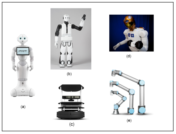
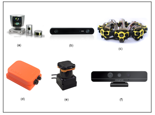
The above are supported robots, starting from Pepper (a), REEM-C (b), Turtlebot (c), Robotnaut (d) and Universal robot (e). In addition, the sensors supported by ROS include LIDAR, SICK laser lms1xx, lms2xx, Hokuyo, Kinect-v2, Velodyne .., for more details, you can see the picture below.

17

Basic understanding of how ROS work:

Basically ROS files are laid out and behave like this, top down in the following order, metapackages, packages, packages manifest, Misc, messages, Services, codes:

18

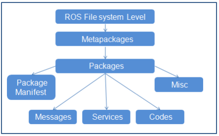
In that package (Metapackages) is a group of packages (packages) related to each other. For example, in ROS there is a total package called Navigation, this package contains all packages related to the movement of the robot, including body movement, wheels, related algorithms such as Kalman, Particle filter. … When we install the master package, it means all the sub-packages in it are also installed.

19

Packages (Packages), here I translate them as packages for easy understanding, the concept of packages is very important, we can say that the package is the most basic atoms that make up ROS. In one package includes, ROSnode, datasets, configuration files, source files, all bundled in one “package”. However, although there are many things in one package, but to work, we only need to care about 2 things in one package, which is the src folder, which contains our source code, and the Cmake.txt file, here is where we declare the libraries needed to execute (compile) code.

Interaction between nodes in ROS

ROS computation graph is a big picture of the interaction of nodes and topics with each other.

In the picture above, we can see that the Master is the nodes that connect all the remaining nodes.

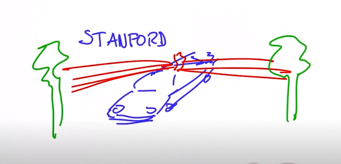
Nodes: ROS nodes are simply the process of using the ROS API to communicate with each other. A robot may have many nodes to perform its communication. For example, a self-driving robot will have the following nodes, node that reads data from Laser scanner, Kinect camera, localization and mapping, node sends speed command to the steering wheel system.

Master: ROS master acts as an intermediate node connecting between different nodes. Master covers information about all nodes running in the ROS environment. It will swap the details of one button with the other to establish a connection between them. After exchanging information, communication will begin between the two ROS nodes. When you run a ROS program, ros_master always must run it first. You can run ros master by -> terminal-> roscore.

Message: ROS nodes can communicate with each other by sending and receiving data in the form of ROS mesage. ROS message is a data structure used by ROS nodes to exchange data. It is like a protocol, format the information sent to the nodes, such as string, float, int …

Topic: One of the methods for communicating and exchanging messages between two nodes is called ROS Topic. ROS Topic is like a message channel, in which data is exchanged by ROS message. Each topic will have a different name depending on what information it will be in charge of providing. One Node will publish information for a Topic and another node can read from the Topic by subcrible to it. Just like you want to watch your videos, you must subcrible your channel. If you want to see which topics you are running on, the command is rostopic list, if you want to see a certain topic see what nodes are publishing or subcrible on it. Then the command is rostopic info / terntopic. If you want to see if there is anything in that topic, type rostopic echo / terntopic.

Service: Service is a different type of communication method from Topic. Topic
uses a publish or subcrible interaction, but in the service, it interacts in a request – response fashion. This is exactly like the network side. One node will act as a server, there is a permanent server
run and when the Node client sends a service request to the server. The server will perform the service and send the result to the client. The client node must wait until the server responds with the result. The server is especially useful when we need to execute something that takes a long time to process, so we leave it on the server, when we need it we call.

Posted in Self-Driving Car

Trajectory Generation

Hybrid A* Pseudocode:

The pseudocode below outlines an implementation of the A* search algorithm using the bicycle model. The following variables and objects are used in the code but not defined there:

  • State(x, y, theta, g, f): An object which stores xy coordinates, direction theta, and current g and f values.
  • grid: A 2D array of 0s and 1s indicating the area to be searched. 1s correspond to obstacles, and 0s correspond to free space.
  • SPEED: The speed of the vehicle used in the bicycle model.
  • LENGTH: The length of the vehicle used in the bicycle model.
  • NUM_THETA_CELLS: The number of cells a circle is divided into. This is used in keeping track of which States we have visited already.

The bulk of the hybrid A* algorithm is contained within the search function. The expand function takes a state and goal as inputs and returns a list of possible next states for a range of steering angles. This function contains the implementation of the bicycle model and the call to the A* heuristic function.

def expand(state, goal):
    next_states = []
    for delta in range(-35, 40, 5): 
        # Create a trajectory with delta as the steering angle using 
        # the bicycle model:

        # ---Begin bicycle model---
        delta_rad = deg_to_rad(delta)
        omega = SPEED/LENGTH * tan(delta_rad)
        next_x = state.x + SPEED * cos(theta)
        next_y = state.y + SPEED * sin(theta)
        next_theta = normalize(state.theta + omega)
        # ---End bicycle model-----

        next_g = state.g + 1
        next_f = next_g + heuristic(next_x, next_y, goal)

        # Create a new State object with all of the "next" values.
        state = State(next_x, next_y, next_theta, next_g, next_f)
        next_states.append(state)

    return next_states

def search(grid, start, goal):
    # The opened array keeps track of the stack of States objects we are 
    # searching through.
    opened = []
    # 3D array of zeros with dimensions:
    # (NUM_THETA_CELLS, grid x size, grid y size).
    closed = [[[0 for x in range(grid[0])] for y in range(len(grid))] 
        for cell in range(NUM_THETA_CELLS)]
    # 3D array with same dimensions. Will be filled with State() objects 
    # to keep track of the path through the grid. 
    came_from = [[[0 for x in range(grid[0])] for y in range(len(grid))] 
        for cell in range(NUM_THETA_CELLS)]

    # Create new state object to start the search with.
    x = start.x
    y = start.y
    theta = start.theta
    g = 0
    f = heuristic(start.x, start.y, goal)
    state = State(x, y, theta, 0, f)
    opened.append(state)

    # The range from 0 to 2pi has been discretized into NUM_THETA_CELLS cells. 
    # Here, theta_to_stack_number returns the cell that theta belongs to. 
    # Smaller thetas (close to 0 when normalized  into the range from 0 to 
    # 2pi) have lower stack numbers, and larger thetas (close to 2pi when 
    # normalized) have larger stack numbers.
    stack_num = theta_to_stack_number(state.theta)
    closed[stack_num][index(state.x)][index(state.y)] = 1

    # Store our starting state. For other states, we will store the previous 
    # state in the path, but the starting state has no previous.
    came_from[stack_num][index(state.x)][index(state.y)] = state

    # While there are still states to explore:
    while opened:
        # Sort the states by f-value and start search using the state with the 
        # lowest f-value. This is crucial to the A* algorithm; the f-value 
        # improves search efficiency by indicating where to look first.
        opened.sort(key=lambda state:state.f)
        current = opened.pop(0)

        # Check if the x and y coordinates are in the same grid cell 
        # as the goal. (Note: The idx function returns the grid index for 
        # a given coordinate.)
        if (idx(current.x) == goal[0]) and (idx(current.y) == goal.y):
            # If so, the trajectory has reached the goal.
            return path

        # Otherwise, expand the current state to get a list of possible 
        # next states.
        next_states = expand(current, goal)
        for next_s in next_states:
            # If we have expanded outside the grid, skip this next_s.
            if next_s is not in the grid:
                continue
            # Otherwise, check that we haven't already visited this cell and
            # that there is not an obstacle in the grid there.
            stack_num = theta_to_stack_number(next_s.theta)
            if closed[stack_num][idx(next_s.x)][idx(next_s.y)] == 0 
                and grid[idx(next_s.x)][idx(next_s.y)] == 0:
                # The state can be added to the opened stack.
                opened.append(next_s)
                # The stack_number, idx(next_s.x), idx(next_s.y) tuple 
                # has now been visited, so it can be closed.
                closed[stack_num][idx(next_s.x)][idx(next_s.y)] = 1
                # The next_s came from the current state, and is recorded.
                came_from[stack_num][idx(next_s.x)][idx(next_s.y)] = current

Now we go to next step:

Implementing Hybrid A*

In this exercise, you will be provided a working implementation of a breadth first search algorithm which does not use any heuristics to improve its efficiency. Your goal is to try to make the appropriate modifications to the algorithm so that it takes advantage of heuristic functions (possibly the ones mentioned in the previous paper) to reduce the number of grid cell expansions required.

Instructions:

  1. Modify the code in ‘hybrid_breadth_first.cpp’ and hit Test Run to check your results.
  2. Note the number of expansions required to solve an empty 15×15 grid (it should be about 18,000!). Modify the code to try to reduce that number. How small can you get it?

Solution:

#include <iostream>
#include <vector>
#include "hybrid_breadth_first.h"

using std::cout;
using std::endl;

// Sets up maze grid
int X = 1;
int _ = 0;

/**
 * TODO: You can change up the grid maze to test different expansions.
 */
vector<vector<int>> GRID = {
  {_,X,X,_,_,_,_,_,_,_,X,X,_,_,_,_,},
  {_,X,X,_,_,_,_,_,_,X,X,_,_,_,_,_,},
  {_,X,X,_,_,_,_,_,X,X,_,_,_,_,_,_,},
  {_,X,X,_,_,_,_,X,X,_,_,_,X,X,X,_,},
  {_,X,X,_,_,_,X,X,_,_,_,X,X,X,_,_,},
  {_,X,X,_,_,X,X,_,_,_,X,X,X,_,_,_,},
  {_,X,X,_,X,X,_,_,_,X,X,X,_,_,_,_,},
  {_,X,X,X,X,_,_,_,X,X,X,_,_,_,_,_,},
  {_,X,X,X,_,_,_,X,X,X,_,_,_,_,_,_,},
  {_,X,X,_,_,_,X,X,X,_,_,X,X,X,X,X,},
  {_,X,_,_,_,X,X,X,_,_,X,X,X,X,X,X,},
  {_,_,_,_,X,X,X,_,_,X,X,X,X,X,X,X,},
  {_,_,_,X,X,X,_,_,X,X,X,X,X,X,X,X,},
  {_,_,X,X,X,_,_,X,X,X,X,X,X,X,X,X,},
  {_,X,X,X,_,_,_,_,_,_,_,_,_,_,_,_,},
  {X,X,X,_,_,_,_,_,_,_,_,_,_,_,_,_,}};

vector<double> START = {0.0,0.0,0.0};
vector<int> GOAL = {(int)GRID.size()-1, (int)GRID[0].size()-1};

int main() {
  cout << "Finding path through grid:" << endl;
  
  // Creates an Empty Maze and for testing the number of expansions with it
  for(int i = 0; i < GRID.size(); ++i) {
    cout << GRID[i][0];
    for(int j = 1; j < GRID[0].size(); ++j) {
      cout << "," << GRID[i][j];
    }
    cout << endl;
  }

  HBF hbf = HBF();

  HBF::maze_path get_path = hbf.search(GRID,START,GOAL);

  vector<HBF::maze_s> show_path = hbf.reconstruct_path(get_path.came_from, 
                                                       START, get_path.final);

  cout << "show path from start to finish" << endl;
  for(int i = show_path.size()-1; i >= 0; --i) {
      HBF::maze_s step = show_path[i];
      cout << "##### step " << step.g << " #####" << endl;
      cout << "x " << step.x << endl;
      cout << "y " << step.y << endl;
      cout << "theta " << step.theta << endl;
  }
  
  return 0;
}
Posted in Self-Driving Car

Implement Practical Filter

Particle Filter Algorithm Steps and Inputs

The flowchart below represents the steps of the particle filter algorithm as well as its inputs.

Particle Filter Algorithm Flowchart

Psuedo Code

This is an outline of steps you will need to take with your code in order to implement a particle filter for localizing an autonomous vehicle. The pseudo code steps correspond to the steps in the algorithm flow chart, initialization, prediction, particle weight updates, and resampling. Python implementation of these steps was covered in the previous lesson.

Initialization

At the initialization step we estimate our position from GPS input. The subsequent steps in the process will refine this estimate to localize our vehicle.

Prediction

During the prediction step we add the control input (yaw rate & velocity) for all particles

Update

During the update step, we update our particle weights using map landmark positions and feature measurements.

Resampling

During resampling we will resample M times (M is range of 0 to length_of_particleArray) drawing a particle i (i is the particle index) proportional to its weight . Sebastian covered one implementation of this in his discussion and implementation of a resampling wheel.

Return New Particle Set

The new set of particles represents the Bayes filter posterior probability. We now have a refined estimate of the vehicles position based on input evidence.

Posted in Docker

Docker Container

Docker là gì ? Kiến thức cơ bản về Docker

Docker là gì ? Kiến thức cơ bản về Docker

Image for post

I. Tại sao phải dùng Docker ?

Việc setup và deploy application lên một hoặc nhiều server rất vất vả từ việc phải cài đặt các công cụ, môi trường cần cho application đến việc chạy được ứng dụng chưa kể việc không đồng nhất giữa các môi trường trên nhiều server khác nhau. Chính vì lý do đó Docker được ra đời để giải quyết vấn đề này.

II. Docker là gì ?

Docker là một nền tảng cho developers và sysadmin để develop, deploy và run application với container. Nó cho phép tạo các môi trường độc lập và tách biệt để khởi chạy và phát triển ứng dụng và môi trường này được gọi là container. Khi cần deploy lên bất kỳ server nào chỉ cần run container của Docker thì application của bạn sẽ được khởi chạy ngay lập tức.

III. Lợi ích của Docker

  • Không như máy ảo Docker start và stop chỉ trong vài giây.
  • Bạn có thể khởi chạy container trên mỗi hệ thống mà bạn muốn.
  • Container có thể build và loại bỏ nhanh hơn máy ảo.
  • Dễ dàng thiết lập môi trường làm việc. Chỉ cần config 1 lần duy nhất và không bao giờ phải cài đặt lại các dependencies. Nếu bạn thay đổi máy hoặc có người mới tham gia vào project thì bạn chỉ cần lấy config đó và đưa cho họ.
  • Nó giữ cho word-space của bạn sạch sẽ hơn khi bạn xóa môi trường mà ảnh hưởng đến các phần khác.

IV. Cài đặt

Link download: tại đây

Chọn bản cài đặt tương ứng với hệ điều hành của bạn và tiến hành cài đặt theo hướng dẫn đối với Linux còn Windows và MacOS thì bạn chỉ cần tải bản cài về và cài đặt như mọi application khác.

Sau khi cài đặt xong để kiểm tra xem cài đặt thành công hay không ?

  • Mở command line:
$ docker version$ docker info$ docker run hello-world

V. Một số khái niệm

Image for post
  • Docker Client: là cách mà bạn tương tác với docker thông qua command trong terminal. Docker Client sẽ sử dụng API gửi lệnh tới Docker Daemon.
  • Docker Daemon: là server Docker cho yêu cầu từ Docker API. Nó quản lý images, containers, networks và volume.
  • Docker Volumes: là cách tốt nhất để lưu trữ dữ liệu liên tục cho việc sử dụng và tạo apps.
  • Docker Registry: là nơi lưu trữ riêng của Docker Images. Images được push vào registry và client sẽ pull images từ registry. Có thể sử dụng registry của riêng bạn hoặc registry của nhà cung cấp như : AWS, Google Cloud, Microsoft Azure.
  • Docker Hub: là Registry lớn nhất của Docker Images ( mặc định). Có thể tìm thấy images và lưu trữ images của riêng bạn trên Docker Hub ( miễn phí).
  • Docker Repository: là tập hợp các Docker Images cùng tên nhưng khác tags. VD: golang:1.11-alpine.
  • Docker Networking: cho phép kết nối các container lại với nhau. Kết nối này có thể trên 1 host hoặc nhiều host.
  • Docker Compose: là công cụ cho phép run app với nhiều Docker containers 1 cách dễ dàng hơn. Docker Compose cho phép bạn config các command trong file docker-compose.yml để sử dụng lại. Có sẵn khi cài Docker.
  • Docker Swarm: để phối hợp triển khai container.
  • Docker Services: là các containers trong production. 1 service chỉ run 1 image nhưng nó mã hoá cách thức để run image — sử dụng port nào, bao nhiêu bản sao container run để service có hiệu năng cần thiết và ngay lập tức.

VI. Dockerfile

– Dockerfile là file config cho Docker để build ra image. Nó dùng một image cơ bản để xây dựng lớp image ban đầu. Một số image cơ bản: python, unbutu and alpine. Sau đó nếu có các lớp bổ sung thì nó được xếp chồng lên lớp cơ bản. Cuối cùng một lớp mỏng có thể được xếp chồng lên nhau trên các lớp khác trước đó.

– Các config :

  • FROM — chỉ định image gốc: python, unbutu, alpine…
  • LABEL — cung cấp metadata cho image. Có thể sử dụng để add thông tin maintainer. Để xem các label của images, dùng lệnh docker inspect.
  • ENV — thiết lập một biến môi trường.
  • RUN — Có thể tạo một lệnh khi build image. Được sử dụng để cài đặt các package vào container.
  • COPY — Sao chép các file và thư mục vào container.
  • ADD — Sao chép các file và thư mục vào container.
  • CMD — Cung cấp một lệnh và đối số cho container thực thi. Các tham số có thể được ghi đè và chỉ có một CMD.
  • WORKDIR — Thiết lập thư mục đang làm việc cho các chỉ thị khác như: RUN, CMD, ENTRYPOINT, COPY, ADD,…
  • ARG — Định nghĩa giá trị biến được dùng trong lúc build image.
  • ENTRYPOINT — cung cấp lệnh và đối số cho một container thực thi.
  • EXPOSE — khai báo port lắng nghe của image.
  • VOLUME — tạo một điểm gắn thư mục để truy cập và lưu trữ data.

VII. Tạo Demo

Tạo file Dockerfile

FROM golang:1.11 AS builderWORKDIR /go/src/docker-demo/COPY . .RUN CGO_ENABLED=0 GOOS=linux go build -a -installsuffix cgo -o docker-demo .FROM alpine:latestWORKDIR /root/COPY — from=builder /go/src/docker-demo .CMD [“./docker-demo”]

Tạo file main.go

package mainimport (   “fmt”)func main() {   fmt.Println(“Learning Docker”)}

Tiến hành build file Dockerfile

$ docker build .
Image for post
$ docker run 4cc010d9d657
Image for post

Kết quả in ra dòng chữ Learning Docker đã được code trong file main.go

VII. Các lênh cơ bản trong docker

  • List image/container:
$ docker image/container ls
  • Delete image/container:
$ docker image/container rm <tên image/container >
  • Delete all image hiện có:
$ docker image rm $(docker images –a –q)
  • List all container hiện có:
$ docker ps –a
  • Stop a container cụ thể:
$ docker stop <tên container>
  • Run container từ image và thay đổi tên container:
$ docker run –name <tên container> <tên image>
  • Stop all container:
$ docker stop $(docker ps –a –q)
  • Delete all container hiện có:
$ docker rm $(docker ps –a –q)
  • Show log a container:
$ docker logs <tên container>
  • Build một image từ container:
$ docker build -t <tên container> .
  • Tạo một container chạy ngầm:
$ docker run -d <tên image>
  • Tải một image trên docker hub:
$ docker pull <tên image>
  • Start một container:
$ docker start <tên container>