Understanding of Convolutional Neural Network (CNN) — Deep Learning

In neural networks, Convolutional neural network (ConvNets or CNNs) is one of the main categories to do images recognition, images classifications. Objects detections, recognition faces etc., are some of the areas where CNNs are widely used.

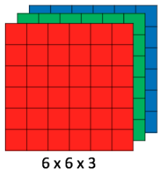
CNN image classifications takes an input image, process it and classify it under certain categories (Eg., Dog, Cat, Tiger, Lion). Computers sees an input image as array of pixels and it depends on the image resolution. Based on the image resolution, it will see h x w x d( h = Height, w = Width, d = Dimension ). Eg., An image of 6 x 6 x 3 array of matrix of RGB (3 refers to RGB values) and an image of 4 x 4 x 1 array of matrix of grayscale image.

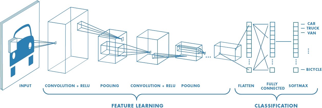
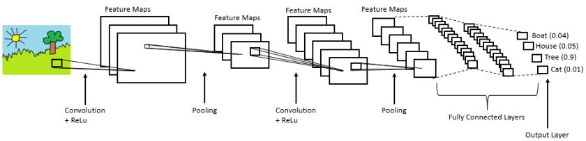
Technically, deep learning CNN models to train and test, each input image will pass it through a series of convolution layers with filters (Kernals), Pooling, fully connected layers (FC) and apply Softmax function to classify an object with probabilistic values between 0 and 1. The below figure is a complete flow of CNN to process an input image and classifies the objects based on values.

Convolution Layer

Convolution is the first layer to extract features from an input image. Convolution preserves the relationship between pixels by learning image features using small squares of input data. It is a mathematical operation that takes two inputs such as image matrix and a filter or kernel.

Consider a 5 x 5 whose image pixel values are 0, 1 and filter matrix 3 x 3 as shown in below

Then the convolution of 5 x 5 image matrix multiplies with 3 x 3 filter matrix which is called “Feature Map” as output shown in below

Convolution of an image with different filters can perform operations such as edge detection, blur and sharpen by applying filters. The below example shows various convolution image after applying different types of filters (Kernels).

Strides

Stride is the number of pixels shifts over the input matrix. When the stride is 1 then we move the filters to 1 pixel at a time. When the stride is 2 then we move the filters to 2 pixels at a time and so on. The below figure shows convolution would work with a stride of 2.

Padding

Sometimes filter does not fit perfectly fit the input image. We have two options:

• Pad the picture with zeros (zero-padding) so that it fits
• Drop the part of the image where the filter did not fit. This is called valid padding which keeps only valid part of the image.

Non Linearity (ReLU)

ReLU stands for Rectified Linear Unit for a non-linear operation. The output is ƒ(x) = max(0,x).

Why ReLU is important : ReLU’s purpose is to introduce non-linearity in our ConvNet. Since, the real world data would want our ConvNet to learn would be non-negative linear values.

There are other non linear functions such as tanh or sigmoid that can also be used instead of ReLU. Most of the data scientists use ReLU since performance wise ReLU is better than the other two.

Pooling Layer

Pooling layers section would reduce the number of parameters when the images are too large. Spatial pooling also called subsampling or downsampling which reduces the dimensionality of each map but retains important information. Spatial pooling can be of different types:

• Max Pooling
• Average Pooling
• Sum Pooling

Max pooling takes the largest element from the rectified feature map. Taking the largest element could also take the average pooling. Sum of all elements in the feature map call as sum pooling.

Fully Connected Layer

The layer we call as FC layer, we flattened our matrix into vector and feed it into a fully connected layer like a neural network.

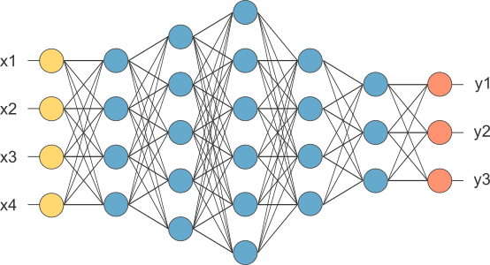
In the above diagram, the feature map matrix will be converted as vector (x1, x2, x3, …). With the fully connected layers, we combined these features together to create a model. Finally, we have an activation function such as softmax or sigmoid to classify the outputs as cat, dog, car, truck etc.,

Summary

• Provide input image into convolution layer
• Choose parameters, apply filters with strides, padding if requires. Perform convolution on the image and apply ReLU activation to the matrix.
• Perform pooling to reduce dimensionality size
• Add as many convolutional layers until satisfied
• Flatten the output and feed into a fully connected layer (FC Layer)
• Output the class using an activation function (Logistic Regression with cost functions) and classifies images.

In the next post, I would like to talk about some popular CNN architectures such as AlexNet, VGGNet, GoogLeNet, and ResNet.

Processing Each Image

In this chapter, the first thing you’ll do is to compute the camera calibration matrix and distortion coefficients. You only need to compute these once, and then you’ll apply them to undistort each new frame. Next, you’ll apply thresholds to create a binary image and then apply a perspective transform.

Thresholding

You’ll want to try out various combinations of color and gradient thresholds to generate a binary image where the lane lines are clearly visible. There’s more than one way to achieve a good result, but for example, given the image above, the output you’re going for should look something like this:

Perspective Transform

Next, you want to identify four source points for your perspective transform. In this case, you can assume the road is a flat plane. This isn’t strictly true, but it can serve as an approximation for this project. You would like to pick four points in a trapezoidal shape (similar to region masking) that would represent a rectangle when looking down on the road from above.

The easiest way to do this is to investigate an image where the lane lines are straight, and find four points lying along the lines that, after perspective transform, make the lines look straight and vertical from a bird’s eye view perspective.

Here’s an example of the result you are going for with straight lane lines:

Now for curved lines

Those same four source points will now work to transform any image (again, under the assumption that the road is flat and the camera perspective hasn’t changed). When applying the transform to new images, the test of whether or not you got the transform correct, is that the lane lines should appear parallel in the warped images, whether they are straight or curved.

Here’s an example of applying a perspective transform to your thresholded binary image, using the same source and destination points as above, showing that the curved lines are (more or less) parallel in the transformed image:

Locate the Lane Lines

Thresholded and perspective transformed image

You now have a thresholded warped image and you’re ready to map out the lane lines! There are many ways you could go about this, but here’s one example of how you might do it:

Line Finding Method: Peaks in a Histogram

After applying calibration, thresholding, and a perspective transform to a road image, you should have a binary image where the lane lines stand out clearly. However, you still need to decide explicitly which pixels are part of the lines and which belong to the left line and which belong to the right line.

Plotting a histogram of where the binary activations occur across the image is one potential solution for this. In the quiz below, let’s take a couple quick steps to create our histogram!

• lane_histogram.py
• solution.py

123456789101112131415161718192021222324import numpy as npimport matplotlib.image as mpimgimport matplotlib.pyplot as plt# Load our image# `mpimg.imread` will load .jpg as 0-255, so normalize back to 0-1img = mpimg.imread(‘warped_example.jpg’)/255print(img.shape)def hist(img): # TO-DO: Grab only the bottom half of the image # Lane lines are likely to be mostly vertical nearest to the car bottom_half = img[img.shape[0]//2:,:] print(bottom_half) # TO-DO: Sum across image pixels vertically – make sure to set `axis` # i.e. the highest areas of vertical lines should be larger values histogram = np.sum(bottom_half, axis = 0) return histogram# Create histogram of image binary activationshistogram = hist(img)# Visualize the resulting histogramplt.plot(histogram)

• RESET QUIZ
• TEST RUN
• SUBMIT ANSWER

Here’s the approach I took.

I take a histogram along all the columns in the lower half of the image like this:

import numpy as np
import matplotlib.pyplot as plt

histogram = np.sum(img[img.shape[0]//2:,:], axis=0)
plt.plot(histogram)

The result looks like this:

Sliding Window

With this histogram we are adding up the pixel values along each column in the image. In our thresholded binary image, pixels are either 0 or 1, so the two most prominent peaks in this histogram will be good indicators of the x-position of the base of the lane lines. We can use that as a starting point for where to search for the lines. From that point, we can use a sliding window, placed around the line centers, to find and follow the lines up to the top of the frame.

Implement Sliding Windows and Fit a Polynomial

As shown in the previous animation, we can use the two highest peaks from our histogram as a starting point for determining where the lane lines are, and then use sliding windows moving upward in the image (further along the road) to determine where the lane lines go.

Split the histogram for the two lines

The first step we’ll take is to split the histogram into two sides, one for each lane line.

import numpy as np
import cv2
import matplotlib.pyplot as plt

# Assuming you have created a warped binary image called "binary_warped"
# Take a histogram of the bottom half of the image
histogram = np.sum(binary_warped[binary_warped.shape[0]//2:,:], axis=0)
# Create an output image to draw on and visualize the result
out_img = np.dstack((binary_warped, binary_warped, binary_warped))*255
# Find the peak of the left and right halves of the histogram
# These will be the starting point for the left and right lines
midpoint = np.int(histogram.shape[0]//2)
leftx_base = np.argmax(histogram[:midpoint])
rightx_base = np.argmax(histogram[midpoint:]) + midpoint

Note that in the above, we also create out_img to help with visualizing our output later on.

Set up windows and window hyperparameters

Our next step is to set a few hyperparameters related to our sliding windows, and set them up to iterate across the binary activations in the image. We have some base hyperparameters below, but don’t forget to try out different values in your own implementation to see what works best!

# HYPERPARAMETERS
# Choose the number of sliding windows
nwindows = 9
# Set the width of the windows +/- margin
margin = 100
# Set minimum number of pixels found to recenter window
minpix = 50

# Set height of windows - based on nwindows above and image shape
window_height = np.int(binary_warped.shape[0]//nwindows)
# Identify the x and y positions of all nonzero (i.e. activated) pixels in the image
nonzero = binary_warped.nonzero()
nonzeroy = np.array(nonzero[0])
nonzerox = np.array(nonzero[1])
# Current positions to be updated later for each window in nwindows
leftx_current = leftx_base
rightx_current = rightx_base

# Create empty lists to receive left and right lane pixel indices
left_lane_inds = []
right_lane_inds = []

Iterate through nwindows to track curvature

Now that we’ve set up what the windows look like and have a starting point, we’ll want to loop for nwindows, with the given window sliding left or right if it finds the mean position of activated pixels within the window to have shifted.

You’ll implement this part in the quiz below, but here’s a few steps to get you started:

1. Loop through each window in nwindows
2. Find the boundaries of our current window. This is based on a combination of the current window’s starting point (leftx_current and rightx_current), as well as the margin you set in the hyperparameters.
3. Use cv2.rectangle to draw these window boundaries onto our visualization image out_img. This is required for the quiz, but you can skip this step in practice if you don’t need to visualize where the windows are.
4. Now that we know the boundaries of our window, find out which activated pixels from nonzeroy and nonzerox above actually fall into the window.
5. Append these to our lists left_lane_inds and right_lane_inds.
6. If the number of pixels you found in Step 4 are greater than your hyperparameter minpix, re-center our window (i.e. leftx_current or rightx_current) based on the mean position of these pixels.

Fit a polynomial

Now that we have found all our pixels belonging to each line through the sliding window method, it’s time to fit a polynomial to the line. First, we have a couple small steps to ready our pixels.

# Concatenate the arrays of indices (previously was a list of lists of pixels)
left_lane_inds = np.concatenate(left_lane_inds)
right_lane_inds = np.concatenate(right_lane_inds)

# Extract left and right line pixel positions
leftx = nonzerox[left_lane_inds]
lefty = nonzeroy[left_lane_inds] 
rightx = nonzerox[right_lane_inds]
righty = nonzeroy[right_lane_inds]

We’ll let you implement the function for the polynomial in the quiz below using np.polyfit.

# Assuming we have `left_fit` and `right_fit` from `np.polyfit` before
# Generate x and y values for plotting
ploty = np.linspace(0, binary_warped.shape[0]-1, binary_warped.shape[0])
left_fitx = left_fit[0]*ploty**2 + left_fit[1]*ploty + left_fit[2]
right_fitx = right_fit[0]*ploty**2 + right_fit[1]*ploty + right_fit[2]

Take note of how we fit the lines above – while normally you calculate a y-value for a given x, here we do the opposite. Why? Because we expect our lane lines to be (mostly) vertically-oriented.

Computer vision (CV) is a process (and a branch of computer science) that involves capturing, processing and analyzing real-world images and video to allow machines to extract meaningful, contextual information from the physical world. Today, computer vision is the foundation and a key means of testing and exploiting deep-learning models that are propelling the evolution of artificial intelligence toward ubiquitous, useful and practical applications. A lot of advancements are expected to occur between 2018 and 2020.

But…what is computer vision?

Back in 1955, researchers assumed they could describe the processes that make up human intelligence and automate them, creating an artificial intelligence (AI). Despite being in a time before 1st demonstration of integrated circuits (IC) in 1958, or 1st commercially available microprocessor by Intel in 1971, or the term graphic processing units (GPU) popularized by Nvidia in 1999, serious researches began and one of the most notable “AI” researches started along three distinct lines: replicating the eye (to see); replicating the visual cortex (to describe); and replicating the rest of the brain (to understand). Along these three distinct lines, various degrees of progresses have been made:

• To See:
  Reinventing the eye is the area with most success. Over the past few decades, sensors and image processors have been created to match or even exceed the human eye’s capabilities. With larger, more optically perfect lenses and nanometer-scaled image sensor and processor, the precision and sensitivity of modern cameras are incredible, especially compared to common human eyes. Cameras can also record thousands of images per second, detect distances and see better in dark environment. However, despite the high fidelity of the outputs, they merely record the distribution of photons coming in a given direction. The best camera sensor ever made couldn’t capture images in 3D until recent hardware breakthroughs (such as flood illuminator with NIR). Modern cameras also provide a much richer and more flexible platform for hardware to work with software.
• To Describe:
  Seeing isn’t enough, but to describe is unfathomably complex. A computer can apply a series of transformations to an image, and therefore discover edges, the objects that these edges imply, and the perspective and movement when presented with multiple pictures, and so on. The processes involve a great deal of math and statistics, and wasn’t made possible until recent advances in parallel computing powered by GPU.
• To Understand:
  Even achieving a toddler’s intelligence has been proven to be extremely complex. Researcher could build a system that recognizes every variety of apples, from every angle, in any situation, at rest or in motion, with bites taken out, anything — and it still wouldn’t be able to recognize an orange. For that matter, it couldn’t even tell you what an apple is, whether it’s edible, how big it is or what they’re used for. Why? Because we barely understand how our minds work: Short and long term memory, input from our other senses, attention and cognition, a billion lessons learned from a trillion interactions with the world, etc. This is not a dead end, but it’s definitely hard to pin down. The past efforts of building a know-it-all expert systems have been proven to be fruitless. A new AI architecture has emerged in the past 5 years or so.

As three key interlocking factors has begun to come together since 2012, the concepts of “context, attention, intention” are slowly evolving into computer vision, a new branch of AI:

• Radical New Hardware:
  Achieved by highly parallel GPU with the rise of foundry-fabless business model (such as TSMC and Nvidia). Liberating IC design and manufacturing from the proprietary-minded IDMs has installed more flexibility into hardware and thus allows software development to prosper. TSMC achieving 28nm mass production in 2012 has been the inflection point. Intel’s 10nm meltdown could further cement this trend.
• Much More Powerful Algorithms:
  Unbinding software development from hardware manufacturing has invited software developers to join the revolution. With then pure software company like Microsoft bursting onto the scene in 1975, programmers have since invented many powerful tools to utilize radical new hardware, and one of the prime examples is deep neural networks (DNNs). We consider today’s DNNs to be smart because they can identify novel patterns in their input streams. Patterns their programmers did not anticipate. DNN performance on image recognition tests (ImageNet) exhibits lower error rates than humans performing the same tests.
• Huge Swatches of Data:
  During the transition from centralized to decentralized architecture, internet was invented. With internet, collecting and integrating large amount of data becomes possible. From the internet, feeding DNNs with big data on powerful GPUs becomes a reality. With more application processors (AP) in personal devices adopting AI-enabled CV, CV applications are expanding along with more available frameworks and tools.

Let’s take a look at some of the currently notable/predictable CV applications on personal devices:

Smartphone: Differentiation Opportunities

AI-driven capabilities enabled by CV have quickly become critical differentiation factors in the saturated smartphone market. These features attempt to transform smartphones from a passive utility tool to a more proactive personal assistant.

The emergence of CV in smartphones is driven by continued investments in AI techniques by major OEMs (Apple, Samsung, Huawei, and Google) and smartphone software, as well as the evolution of image sensors (Sony), image processing units (Sony and in-house ASICs) and modules’ miniaturization (Largan, etc.). For the past couple of years, new smartphones has been characterized by continued sophistication in cameras, with higher resolutions to capture more data to improve overall accuracy of visual recognition applications and integration of 3D depth-sensing technology to enhance the reliability of facial recognition. Google started it with its Tango-enabled phones, Lenovo Phab 2 and ASUS ZenFone AR, but failed to elaborate. Last year (2017), Apple introduced 3D sensing in the iPhone X, donned “TrueDepth” as part of the front-facing camera setup. Apple’s move has led to a rush in 3D sensing adoption. 3D-sensing technology is still far from mainstream, but increased availability and affordability of 3D sensors for phones is expected to continue and make it into more Android smartphones between 2018 and 2019.

If CV in smartphone follows mobile payment’s (by NFC) footstep, all premium smartphones would likely include CV capability by 2020 and 30% to 50% of non-premium smartphones would have the function before 2022. Facial or gesture recognition could become one of the standard authentication mechanisms and other CV apps would emerge as people get used to it. Here’s some directions for CV applications:

• Optimize Camera Settings:
  Huawei uses the AI function on its Kirin 970 chip to recognize objects and scenarios to optimize the camera settings automatically. The AI-enabled camera can recognize more than 500 scenarios across 19 categories (food, group, sunset, greenery and night shot, etc.) and will adjust camera-setting features such as exposure, International Organization for Standardization (ISO) and color saturation or contrast, in real time. This enables users to get the best shot for each category. It is also able to perform object recognition linked to shopping applications and text translation based on an application developed with Microsoft Translator.
• Augmented Reality (AR):
  Apple is already using the TrueDepth system in the iPhone X to produce Animoji, its animated emoji feature, for social networking. In the future, Apple will likely expand on AR applications. Apple acquired computer vision startup Ragaind, whose CV API can analyze photos and recognize in pictures faces, their gender, age and emotions. In 2016, Apple acquired the startup Emotient, which uses AI to recognize people’s emotions from facial expressions (the technology has probably been applied to Animoji already).
• Query and Assistant:
  Google Lens, integrating Google’s expertise in CV and machine learning (ML), along with its extensive knowledge graph, can perform visual search. Using a smartphone camera, Lens detects an object, landmark or restaurant, recognizes what it sees, and offers information and specific actions about what it detects. At Google I/O 2018, Google announced enhancements to Lens, such as smart text selection and search. It also announced style match (if you see an item you like while shopping, Lens can show not only reviews but other similar shopping options or similar items to the one you like). However, Google Lens has received quite a few harsh reviews so far, likely due to the technology’s immaturity.
• Health and Record Book:
  Samsung has been exploring CV with Bixby Vision. One of the use cases is food calories calculation. Ideally, Samsung’s Bixby Vision could calculate how much calories you consume by reviewing photos of your meal. For those who have been using MyFitnessPal with Asian dishes, trying to find matches and record calories is a PITA. Some other emerging well-being applications , applications such as Calorie Mama , AI has been employed to help manage and advise on diet and calorie intake, and monitor food composition, from food photos using deep learning and computer vision.

The advancements in computer vision and smartphones will likely have the most far-reaching impact. e-Commerce is also an area worth watching. CV could provide AR function for home décor/furnishing applications or clothes fitting. The biggest advantage of brick-and-mortar could erode fast.

Head-Mounted Display (HMD): Immersive Experiences

CV can enhance immersive experiences via eye and position tracking, gesture recognition, and by mapping virtual environments. It will also help with realistic overlaying of virtual things in the real world in mixed reality, as well as enabling object or location recognition. However, HMD still only plays in a niche market with relatively few applications. To imagine how HMD could utilize computer vision to change our life, we have to look into the progresses of several major participants:

• Qualcomm: Turning Smartphone into HMD:
  Qualcomm has Vision Intelligence Platform to support edge/on-device computing for camera processing and machine learning. With in-house CV software development kits, Qualcomm chips (currently on 10nm) can support VR cameras, robotics, and smartphone/wearable cameras. Qualcomm has also partnered with SenseTime(for face, image and object recognition, but as a Chinese AI startup, some privacy concern might emerge), Pilot.ai(for detection, classifications and tracking of objects/actions) and MM Solutions (for image-quality tuning services, acquired by ThinderSoft, another Chinese company which could bring up privacy concern).
• Facebook: Standalone HMD via Oculus Acquisition
  Since Facebook acquired Oculus, it has been investing in CV in the last two years. Facebook acquired 3 companies to boost its efforts in CV: Surreal Vision (real-time 3D sense reconstruction of real things in a virtual world), Zurich Eye (enabling machines to navigate in any space), Fayteq (adding digital images into videos).
• Microsoft: Xbox as a Market?
  Next version of HoloLens is expected in 2019 and should support cloud-based CV that will be capable of recognizing objects in AR. Other HMD providers from the Microsoft ecosystem could be offering new devices for MR with CV toward the end of 2019 to support next-generation Xbox (expected to hit market in 2020).

CV is a major enabler for creating more engaging customer experiences on HMDs. It reduces the invasive nature of advertisements. For more corporate use such as using HMD for employee training or collaborating on design or experiments, it could take years to create a viable common platform before collecting enough data. However, the internet has proven that advertisement alone is enough to drive massive innovation. The ability to offer location-specific experiences and services through CV would also help improve user experience for HMD.

Personal Robots: a Visual Touch to Non-Optical Sensory Data

Currently, iRobot is probably the first thing that comes up when we think about personal robot, but cleaning bot is neither smart or multi-functional. It’s far from the humanoid that we imagine. Personal robots today are confined within the data generated by their sensors. Some of the more versatile robots, like Honda’s ASIMO in the graph above, cannot really learn despite being equipped with some cameras.

Computer vision could change all these.

CV complements sensory data in personal robots. It will enrich how personal robots can interact with the environment. CV is enabled in robots via camera mapping, 3D sensor mapping and simulations localization and mapping algorithms. It can be used for edge detection for rooms, furniture and stairs, and for floor plan modeling for cleaning robots. With CV, personal service robots could recognize different members of the family to support individual interactions and personal contexts, and assisting elderly people or people with disabilities in their own homes or in care homes. Remote healthcare for diagnostic and ongoing treatments would also become more reliable with CV and ML. At CES 2018, many robots with some implementations of CV were demonstrated. Many more should come in the next few years.

Voice-Enabled Personal Assistant (VPA): Multi-modal Speakers

Since its introduction in 2014, more than 12,000 providers have leveraged the functionality of VPA speakers to deliver services, most of them connected home solutions around the Amazon Alexa skill set as Google and Apple were late to the party.

Originally, VPA focuses on audio rendering capabilities and connectivity to cloud-based music services, and as such, these speakers have proven to be a popular music player in the home. However, doubling down on the proven acceptance of these products, 2nd-generation VPAs are now adding cameras and screens to transform into AI-based VPAs.

With Apple’s HomdPod yet to prove its usefulness, VPA market is now dominated by Amazon with Google as the only worthy challenger, especially in the AI-based VPA field:

• Amazon: the Clear Leader
  Amazon started the VPA trend with the introduction of Amazon Echo in 2014. It features far-field voice capturing, wireless (Wi-Fi and Bluetooth) connectivity, and high quality built-in loudspeakers for audio rendering. It was a huge success, but the AI focuses on voice not visual. In 2017, Amazon announced the Echo Show for the Alexa platform, incorporating a 7-inch LCD screen and a camera. Later that year, the Echo Spot began shipping with a circular 2.5-inch screen and camera. The biggest purpose of screens and cameras was to enable videoconferencing applications to improve the customer experience, but these two devices also serve as the basis of training Alexa’s CV capabilities. The Echo Look then shows how camera-enabled Alexa devices can be developed into CV-enabled platforms (which became available on 2018/6/6). The built-in camera can capture a user’s full body image and apply AI to create effects such as a blurred background. More importantly, cloud-based AI can analyze the attire of the user and make the appropriate shopping recommendations for similar styles. Oddly, the Echo Look does not have a screen. As a result, the rendering of the captured images and the shopping suggestions have to come from a connected device such as a smartphone running the Echo Look app, leaving room for future improvement. Imagine if mixed reality is possible with a built-in projector on next-gen Echo Look, Echo Look could project recommended clothes on your body with the camera recording it for you to review the look or share with others for opinion in real-time.
• Google: Leader in AI, Follower in VPA
  So far, Google’s participation in VPA has followed Android’ footstep: it hasn’t announced any multimodal Pixel VPA yet, but instead, it relies on hardware partners such as LG, Lenovo and others to provide multimodal devices. At CES 2018, LG announced the LG WK9, a ThinQ-enabled smart speaker device with an 8-inch touch display and camera for videoconferencing for Google Assistant. Lenovo announced its Smart Display with 8-inch or 10-inch screen options and a camera, also running Google Assistant. These device isn’t utilizing CV capabilities yet, but with Qualcomm S624 as application processor (which is designed not only for video applications in connected hubs, but also for device-based AI processing), one can imagine that these devices will have CV either through driver update or in next iteration. However, without clear “profitable” use cases as these hardware partners cannot really make money from retail, the potential remains somewhat undeveloped.

Drone: CV to Elevate Freight and Provide Bridge to Last-Mile

Computer vision capabilities are increasingly being leveraged in drones with a potentially transformational impact in both personal and commercial drone applications.

The biggest impact could come from ambitions of drones for delivery. CV can help enable improving autonomous navigation beyond GPS in situations of pilot assistance in low visibility. CV can also enhance obstacle/collision avoidance and analysis of the best route calculation as CV, AI (ML) and simultaneous localization and mapping have been intertwined to enable 3D mapping and structure reconstruction, object detection and tracking, awareness of context, terrain analysis and path planning.

For shipping, CV could also act like Apple’s FaceID in authentication. One of the biggest concern for drone last-mile delivery is that someone could ninja your package. Using CV (if users have pre-registered forfacial recognition), identifying the right receiver won’t be a problem anymore. However, to enable this function, 5G might be a must.

Connected Home: Personalized Internet of Things

Google is using CV in its Nest Cam IQ and Nest Cam IQ Outdoor to enable recognition of specific family members or friends, as well as the Sightline feature that identifies specific events in the video footage. The company also recently launched a smart camera, Google Clips, which can be placed around the house and will use algorithms and CV to capture “special moments.”

Nonetheless, cameras in connected-home appliances haven’t really evolved beyond home security features (which could provoke privacy concern as parents might be using these cameras by taking video footage without permission). Google introduced Nest Hello doorbell with a wide-angle camera for video able to perform facial recognition, which could be used as a means to unlock (or not to unlock) the door.

Computer vision adds a natural way for users to interact with the digital and physical worlds around them. It is enabling new interaction models for devices with users and the environment around them, but there are two main concerns around CV.

The first one is technological. As a young technology, there is no definitive algorithm for CV, and most of the popular algorithms out there are proprietary. The proprietary algorithms restricted CV capabilities on specific devices and use cases. For example, iRobot’s cleaning bots won’t share CV with your home security cameras. Facial recognition for a family in iPhones would coordinate with Amazon’s VPAs.

The second major concern is around privacy and country/region-specific regulations (such as GDPR in Europe). Many devices — HMDs and personal robots — with CV will collect a lot of data, images, video around individual consumers, a household, their routine, personal data information, information about kids, and patient information in a hospital’s reception area. The limitation of data retrieval could hamper the development of CV and AI.

Computer vision would be the closest AI that we will experience on a daily basis. Visual processing unit (VPU) for CV, 5G development and the deployment of edge computing will help CV form our future in the next few years.

Reference: Michael Wang-Medium